Welcome to Skyzhou's Notes
ようこそいらっしゃいました!
目前已经有的笔记:
有些笔记可能 $\LaTeX$ 一下子加载不出来,需要手动刷新一下
非常抱歉!
CSC3001 Discrete Mathematics
L0 Introduction
Main Course Topics
- Propositional Logic
- Sets, First-Order Logic
- Methods of Proofs
- Mathematical Induction
- Recursion
- Greatest Common Divisors
- Modular Arthmetic
- Chinese Remainder Theorem
- Graphs
- Graph Matching
- Graph Coloring
- Combinatorial Proofs and its Principles
- Counting by Mapping
- Cardinality
L1 Propositional Logic
Statement (Proposition)
A Statement is a sentence that is either True or False.
e.g. $2+2=4 \to \text{True}$
Non e.g. $x+y>0$, cause they are true for some values of $x$ and $y$, but false for others.
Logic Operators
NOT $\lnot$
Alternative notation: $\lnot P = \overline{P}$
| $P$ | $\lnot P$ |
|---|---|
| T | F |
| F | T |
AND $\land$
| $P$ | $Q$ | $P\land Q$ |
|---|---|---|
| T | T | T |
| T | F | F |
| F | T | F |
| F | F | F |
OR $\lor$
| $P$ | $Q$ | $P\lor Q$ |
|---|---|---|
| T | T | T |
| T | F | T |
| F | T | T |
| F | F | F |
XOR $\oplus$
Exclusive OR
| $P$ | $Q$ | $P\oplus Q$ |
|---|---|---|
| T | T | F |
| T | F | T |
| F | T | T |
| F | F | F |
De Morgan's Laws
Logical Equivalence: Two statements have the same truth table.
De Morgan's Laws:
$$ \lnot (P \land Q) \equiv \lnot P \lor \lnot Q $$ $$ \lnot (P \lor Q) \equiv \lnot P \land \lnot Q $$
Tautology and Contradiction
A tautology is a statement that is always true.
- e.g. $P \lor \lnot P$
A contradiction is a statement that is always false. (Negation of a tautology)
- e.g. $P \land \lnot P$
Conditinal Statement
If $\to$
If P then Q: $P \to Q \equiv \lnot P \lor Q$
| $P$ | $Q$ | $P \to Q$ |
|---|---|---|
| T | T | T |
| T | F | F |
| F | T | T |
| F | F | T |
Convention: If we don't say anything wrong, then it is not false, and thus true.
Negation of If-Then: $\lnot(P \to Q) \equiv P \land \lnot Q$
Contrapositive: The contrapositive of $P \to Q$ is $\lnot Q \to \lnot P$
$$ P \to Q \equiv \lnot P \lor Q \equiv Q \lor \lnot P \equiv \lnot Q \to \lnot P $$
If and Only If $\iff$
P if Q means "if Q then P", or "Q implies P". We also say Q is a sufficient condition for P.
P only if Q means "if P then Q", or "P implies Q". We also say Q is a necessary condition for P.
P if and only if (iff) Q means P and Q are logically equivalent.
| $P$ | $Q$ | $P \iff Q$ |
|---|---|---|
| T | T | T |
| T | F | F |
| F | T | F |
| F | F | T |
$$ P \iff Q \equiv (P \to Q) \land (Q \to P) \equiv (P \to Q) \land (\lnot P \to \lnot Q) $$
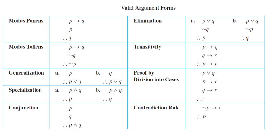
Argument
An argument is a sequence of statements.
All statements but the final one are called assumptions or hypothesis.
The final statement is called the conclusion.
An argument is valid if: whenever all the assumptions are true, then the conclusion is true. Or we say the conclusion follows from the assumptions.
L2 Sets
Basic Definitions
Defining Sets
Set: A set is an unordered collection of distinct objects.
Elements / Members: The objects in a set are called the elements or members of the set S, and we say S contains its elements.
e.g. $S=\{2,3,5,7\} = \{3,7,2,5\}$ (Unordered)
Alternatively, we use the notation $\{x \in A | P(x)\}$ to define the set as the set of elemets, $x$, in $A$ such that $x$ satisfies property $P$.
Classical Sets
- $\mathbb{Z}$: The set of all integers
- $\mathbb{Z^+}$: The set of all positive integers
- $\mathbb{Z^-}$: The set of all negative integers
- $\mathbb{N}$: The set of all nonnegative integers
- $\mathbb{R}$: The set of all real numbers
- $\mathbb{Q}$: The set of all rational numbers
- $\mathbb{C}$: The set of all complex numberse
Membership
The most basic question in set theory is whether an element is in a set.
- $A \subseteq B$: $A$ is an subset of $B$
- $A = B$: $A$ is equal to $B$
- $A \subset B$: $A$ is an proper subset of $B$
Operations on Sets
Basic Operations on Sets
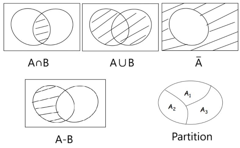
Intersection: $A \cap B = \{x \in U | x \in A \text{ and } x \in B\}$
Two sets are said to be disjoint if their intersection is an empty set.
Union: $A \cup B = \{x \in U | x \in A \text{ or } x \in B\}$
And we have $|A \cup B| = |A|+|B| - |A \cap B|$
Complement: $\overline{A} = A^c = \{x \in U | x \notin A\}$
And if $A \subseteq B$, then $\overline{B} \subseteq \overline{A}$
Difference: $A - B = \{ x \in U | x \in A \text{ and }x \notin B \}$
And we have $|A-B| = |A| - |A \cap B|$
Big set operators: $$ \begin{align*} \bigcup_{i=0}^n A_i &= \{ x \in A_i \text{ for at least one } i = 0, 1, 2, \cdots, n \} \\ \bigcap_{i=0}^n A_i &= \{ x \in A_i \text{ for all } i = 0, 1, 2, \cdots, n \} \end{align*} $$
Partition of Sets
Partition: A collection of nonempty sets $\{ A_1, A_2, \cdots, A_n \}$ is a partition of a set A if and only if $$ \begin{align*} & A = A_1 \cup A_2 \cup \cdots \cup A_n \\ & A_1, A_2, \cdots, A_n \text{ are mutually disjoint (or pairwise disjoint)} \end{align*} $$
Cartesian Products
Cartesian Products: Given two sets $A$ and $B$, the Cartesian product $A \times B$ is the set of all ordered pairs $(a,b)$, where $a$ is in $A$ and b is in $B$. That is: $$ A \times B = \{(a,b) | a \in A, b \in B\} $$
e.g. Let $A = \{ a, b, c, \cdots, z \}$. Let $B = \{ 0, 1, 2, \cdots, 9 \}$. Then $A \times B = \{ (a,1), (a,2), \cdots, (a, 9), (b, 1), (b, 2), \cdots, (z, 9) \}$
Well...It may seems a bit like the outer product of two vectors is a matrix, but in a set.
Set Identities
Set Laws
Let $A$, $B$ and $C$ be subsets of a universal set $U$, and we have:
- Commutative Law
- $A \cup B = B \cup A$
- $A \cap B = B \cap A$
- Associative Law
- $(A \cup B) \cup C = A \cup (B \cup C)$
- $(A \cap B) \cap C = A \cap (B \cap C)$
- Distributive Law
- $A \cup (B \cap C) = (A \cup B) \cap (A \cup C)$
- $A \cap (B \cup C) = (A \cap B) \cup (A \cap C)$
- Identity Law
- $A \cup \emptyset = A$
- $A \cap U = A$
- Complement Law
- $A \cup A^c = U$
- $A \cap A^c = \emptyset$
- De Morgan's Law
- $(A \cup B)^c = A^c \cap B^c$
- $(A \cap B)^c = A^c \cup B^c$
- Set Difference Law
- $A - B = A \cap B^c$
L3 First-order Logic
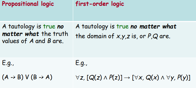
Quantifiers
Predicates
Predicate: Propositions (i.e. statments) with variables.
- e.g. $P(x, y): x + 2 = y$
The domain of a variable is the set of all values that may be substituted in place of the variable.
The truth of a quantified statement depends on the domain.
The Universal Quantifier $\forall$
$\forall x$: For ALL $x$
- e.g. $\forall x, x^2 \geq x$
The Existential Quantifier $\exists$
$\exists x$: There EXISTS some $x$ (perhaps one)
- e.g. $\exists x \in \mathbb{Z}^+, x=x^2$
e.g. How to write prime(p) ?
A prime number is a natural number greater than $1$ that has no positive divisors other than $1$ and itself.
- Conditions: $p \not= ab$
- Variables: $p, a, b$
- Domains: $p, a, b > 1, p, a, b \in \mathbb{Z}$
- Add quantifiers and reconcile the order:
$$ (p > 1) \land (p \in \mathbb{Z}) \land (\forall a, b, \in \mathbb{Z}^+, (p \not= ab) \lor (a=1) \lor (a=p)) $$
Negation
One simple equivalence: $$ \lnot \forall x, P(x) \equiv \exists x, \lnot P(x) $$ e.g. Not every like you = There exists someone who doesn't like you.
Multiple Quantifiers
The order of quantifiers is very important.
Arguments of Quantified Statements
Predicate Calculus Validity
A quantified argument is valid if the conclusion is true whenever the assumptions are true.
Arguments with Quantified Statements
Universal Instantiation: $$ \begin{align*} & \forall x , P(x) \\ \therefore \ & P(a) \end{align*} $$
Universal Modus Ponens $$ \begin{align*} & \forall x , (P(x) \to Q(x)) \\ & P(a) \\ \therefore \ & Q(a) \end{align*} $$
Universal Modus Tollens: $$ \begin{align*} & \forall x, P(x) \to Q(x) \\ & \lnot Q(A) \\ \therefore \ & \lnot P(A) \end{align*} $$
Universal Generalization: $$ \frac{A \to R(c)}{A \to \forall x , R(x)} \qquad \\ \text{(valid rule, provided $c$ is independent of $A$)} $$
CSC3200 Data Structures and Advanced Programming
Introduction
Teaching C++ first.
Then data sturctures.
Assignment 1
Trigonometric Functions
Implement some of the trigonometric functions from scratch without using any mathematical functions from STL.
student_math.h
#ifndef STUDENT_MATH_H
#define STUDENT_MATH_H

namespace student_std {
    double sin(double x); //x is an angle in radian
    double sin_deg(double x); //x is an angle in degree
    double cos(double x); //x is an angle in radian
    double cos_deg(double x); //x is an angle in degree
    double tan(double x); //x is an angle in radian
    double tan_deg(double x); //x is an angle in degree
    double cot(double x); //x is an angle in radian
    double cot_deg(double x); //x is an angle in degree
}

#endif
student_math.cpp
#include "student_math.h"

const double pi = 3.1415926535897932384626;
const double esp = 1e-8;

double toRadian(double x) {
    return pi*x/180.0;
}

double dcmp(double x) {
    return (x < -esp ? -1 : (x > esp ? 1 : 0));
}

double fabs(double x) {
    return (dcmp(x) == -1 ? -x : x);
}

double TrigonometricLagrange(double x, bool issin) {
    while(x > 2.0*pi) x -= 2.0*pi;
    while(x < -2.0*pi) x += 2.0*pi;
    double numerator = 1, denominator = 1;
    double timescnt = 1;
    if(issin) {
        numerator = x;
        timescnt = 2;
    }
    double current = numerator/denominator, last = numerator/denominator;
    double re = current;
    while(fabs(current) > esp) {
        current = current*x*x/(timescnt)/(timescnt+1.0)*(-1.0);
        timescnt += 2;
        re += current;
    }
    return (fabs(re) > esp ? re : 0);
}

namespace student_std {
    double sin(double x) {
        return TrigonometricLagrange(x, 1);
    }
    double sin_deg(double x) {
        return sin(toRadian(x));
    }
    double cos(double x) {
        return TrigonometricLagrange(x, 0);
    }
    double cos_deg(double x) {
        return cos(toRadian(x));
    }
    double tan(double x) {
        return sin(x)/cos(x);
    }
    double tan_deg(double x) {
        return sin(toRadian(x))/cos(toRadian(x));
    }
    double cot(double x) {
        return 1.0/tan(x);
    }
    double cot_deg(double x) {
        return 1.0/tan(toRadian(x));
    }
}
String
Implement a C++ string class from scratch without using STL.
student_string.h
#ifndef STUDENT_STRING_H
#define STUDENT_STRING_H

#define MAXLEN 256
namespace student_std {
    class string {
        public:
            string();
            string(const char* str);
            string(string const&);
            ~string();
            int get_strlen() const;
            const char* get_c_str() const;
            void strcat(string const&);
            string& operator=(string const&);
            string& operator+=(string const&);
            char& operator[](int);
            const char& operator[](int) const;
            void to_upper();
            void to_lower();
            void strcopy(string const&);
            bool equals(string const&) const;
            bool equals_ignore_case(string const&) const;
            void trim(); // Removes spaces ' ' from beginning and end
            bool is_alphabetic() const;
        private: // hint
            char c_str[MAXLEN];
            int strlen;
    };
}

#endif
student_string.cpp
#include "student_string.h"

namespace student_std {
    string::string() {
        this->c_str[0] = '\0';
        this->strlen = 0;
    }

    string::string(const char* str) {
        int len = 0;
        while(str[len] != '\0') {
            len++;
        }
        this->strlen = len;
        for(int i = 0; i <= len; i++) {
            this->c_str[i] = str[i];
        }
    }

    string::string(string const& str) {
        this->strlen = str.strlen;
        for(int i = 0; i <= this->strlen; i++) {
            this->c_str[i] = str.c_str[i];
        }
    }

    string::~string() {}

    int string::get_strlen() const {
        return this->strlen;
    }

    const char* string::get_c_str() const {
        return this->c_str;
    }

    void string::strcat(string const& str) {
        int len = this->strlen;
        for(int i = 0; i <= str.strlen; i++) {
            this->c_str[i+len] = str.c_str[i];
        }
        this->strlen = len+str.strlen;
    }

    string& string::operator=(string const& str) {
        if(this == &str) {
            return *this;
        }
        this->strlen = str.strlen;
        for(int i = 0; i <= this->strlen; i++) {
            this->c_str[i] = str.c_str[i];
        }
        return *this;
    }

    string& string::operator+=(string const& str) {
        this->strcat(str);
        return *this;
    }

    char& string::operator[](int i) {
        return this->c_str[i];
    }

    const char& string::operator[](int i) const {
        return this->c_str[i];
    }

    void string::to_upper() {
        for(int i = 0; i < this->strlen; i++) {
            if(this->c_str[i] >= 'a' && this->c_str[i] <= 'z') {
                this->c_str[i] = char(c_str[i]+('A'-'a'));
            }
        }
    }

    void string::to_lower() {
        for(int i = 0; i < this->strlen; i++) {
            if(this->c_str[i] >= 'A' && this->c_str[i] <= 'Z') {
                this->c_str[i] = char(c_str[i]+('a'-'A'));
            }
        }
    }

    void string::strcopy(string const& str) {
        *this = str;
    }

    bool string::equals(string const& str) const {
        if(this->strlen != str.strlen) return false;
        for(int i = 0; i < this->strlen; i++) {
            if(this->c_str[i] != str.c_str[i]) return false;
        }
        return true;
    }

    bool string::equals_ignore_case(string const& str) const {
        string a = *this, b = str;
        a.to_lower();
        b.to_lower();
        return a.equals(b);
    }

    void string::trim() {
        int l = 0, r = this->strlen-1;
        while(this->c_str[l] == ' ') {
            l++;
        }
        while(this->c_str[r] == ' ') {
            r--;
        }
        for(int i = 0; i < r-l+1; i++) {
            this->c_str[i] = this->c_str[i+l];
        }
        for(int i = r-l+1; i <= this->strlen; i++) {
            this->c_str[i] = '\0';
        }
        this->strlen = r-l+1;
    }

    bool string::is_alphabetic() const {
        for(int i = 0; i < this->strlen; i++) {
            if(!((this->c_str[i] >= 'a' && this->c_str[i] <= 'z') || (this->c_str[i] >= 'A' && this->c_str[i] <= 'Z'))) {
                return false;
            }
        }
        return true;
    }
}
Assignment 2
Vector
Implement a C++ vector (dynamic array) from scratch without using STL.
student_vector.h
#ifndef STUDENT_VECTOR_H
#define STUDENT_VECTOR_H

#include <cstddef>
#include <cassert>
#include <stdexcept>
#include <iterator>

namespace student_std {
    template <typename T>
    class vector {

        public:
            using size_type = std::size_t;
            using difference_type = std::ptrdiff_t;
            using value_type = T;

        private:
            T* s;
            size_type sz;
            size_type cap;

            void reallocate(size_type newcap) {
                if(newcap < sz) newcap = sz;
                T* news = new T[newcap];
                for(size_type i = 0; i < sz; i++) {
                    news[i] = s[i];
                }
                delete[] s;
                s = news;
                cap = newcap;
            }

        public:
            vector() {
                s = nullptr;
                sz = 0;
                cap = 0;
            }

            vector(const vector& other) {
                s = nullptr;
                sz = other.sz;
                cap = other.cap;
                s = new T[cap];
                for(size_type i = 0; i < sz; i++) {
                    s[i] = other.s[i];
                }
            }

            vector& operator= (const vector& other) {
                if(this == &other) return *this;
                delete[] s;
                sz = other.sz;
                cap = other.cap;
                s = new T[cap];
                for(size_type i = 0; i < sz; i++) {
                    s[i] = other.s[i];
                }
                return *this;
            }

            ~vector() {
                delete[] s;
            }

            size_type size() const {
                return sz;
            }

            size_type capacity() const {
                return cap;
            }

            bool empty() const {
                return sz == 0;
            }

            const T* data() const {
                return s;
            }

            const T& at(size_type p) const {
                if(p >= sz) throw std::out_of_range("vector::at out of range");
                else return s[p];
            }

            const T& operator[] (size_type p) const {
                assert(p >= 0 && p < sz);
                return s[p];
            }

            const T& front() const {
                assert(sz > 0);
                return s[0];
            }

            const T& back() const {
                assert(sz > 0);
                return s[sz-1];
            }

            void reserve(size_type newcap) {
                if(newcap > cap) {
                    reallocate(newcap);
                }
            }

            void push_back(const T& val) {
                if(sz == cap) {
                    size_type newcap = (cap == 0 ? 1 : cap * 2);
                    reserve(newcap);
                }
                s[sz] = val;
                sz++;
            }

            void pop_back() {
                assert(sz > 0);
                sz--;
            }

            void resize(size_type newsz, const T& val) {
                if(newsz > cap) {
                    reserve(newsz);
                }
                if(newsz > sz) {
                    for(size_type i = sz; i < newsz; i++) {
                        s[i] = val;
                    }
                }
                sz = newsz;
            }

            void resize(size_type newsz) {
                resize(newsz, T());
            }

            void clear() {
                sz = 0;
            }

            void swap(vector& other) {
                std::swap(s, other.s);
                std::swap(sz, other.sz);
                std::swap(cap, other.cap);
            }

            T* data() {
                return s;
            }

            T& at(size_type p) {
                if(p >= sz) throw std::out_of_range("vector::at out of range");
                else return s[p];
            }

            T& operator[] (size_type p) {
                assert(p >= 0 && p < sz);
                return s[p];
            }

            T& front() {
                assert(sz > 0);
                return s[0];
            }

            T& back() {
                assert(sz > 0);
                return s[sz-1];
            }

        public:
            class iterator {
                public:
                    using difference_type = std::ptrdiff_t;
                    using value_type = T;
                    using pointer = T*;
                    using reference = T&;
                    using iterator_category = std::random_access_iterator_tag;

                private:
                    pointer ptr;

                public:
                    iterator() {
                        ptr = nullptr;
                    }

                    iterator(pointer p) {
                        ptr = p;
                    }

                    reference operator*() const {
                        return *ptr;
                    }

                    pointer operator->() const {
                        return ptr;
                    }

                    iterator& operator++() {
                        ptr++;
                        return *this;
                    }

                    iterator operator++(int) {
                        iterator tmp = *this;
                        ptr++;
                        return tmp;
                    }

                    iterator& operator--() {
                        ptr--;
                        return *this;
                    }

                    iterator operator--(int) {
                        iterator tmp = *this;
                        ptr--;
                        return tmp;
                    }

                    iterator& operator+=(difference_type num) {
                        ptr += num;
                        return *this;
                    }

                    iterator& operator-=(difference_type num) {
                        ptr -= num;
                        return *this;
                    }

                    iterator operator+(difference_type num) const {
                        return iterator(ptr+num);
                    }

                    iterator operator-(difference_type num) const {
                        return iterator(ptr-num);
                    }

                    difference_type operator-(const iterator& other) const {
                        return ptr-other.ptr;
                    }

                    bool operator==(const iterator& other) const{
                        return ptr == other.ptr;
                    }

                    bool operator!=(const iterator& other) const{
                        return ptr != other.ptr;
                    }

                    bool operator<=(const iterator& other) const{
                        return ptr <= other.ptr;
                    }

                    bool operator>=(const iterator& other) const{
                        return ptr >= other.ptr;
                    }

                    bool operator<(const iterator& other) const{
                        return ptr < other.ptr;
                    }

                    bool operator>(const iterator& other) const{
                        return ptr > other.ptr;
                    }
            };

        public:
            iterator begin() {
                return iterator(s);
            }

            iterator end() {
                return iterator(s+sz);
            }

            iterator erase(iterator it) {
                assert(it >= begin() && it < end());
                T* p = &(*it);
                for(T* i = p; i+1 < s+sz; i++) {
                    *i = *(i+1);
                }
                sz--;
                return iterator(p);
            }

            iterator erase(iterator it1, iterator it2) {
                assert(it1 >= begin() && it1 < it2 && it2 <= end());
                T* p1 = &(*it1);
                T* p2 = &(*it2);
                size_type erasecnt = p2 - p1;
                for(T* i = p1; i+erasecnt < s + sz; i++) {
                    *i = *(i+erasecnt);
                }
                sz -= erasecnt;
                return iterator(p1);
            }

            iterator insert(iterator it, const T& val) {
                assert(it >= begin() && it <= end());
                size_type p = it - begin();
                if(sz == cap) reserve(cap == 0 ? 1 : cap * 2);
                it = iterator(s + p);
                for(size_type i = sz; i > p; i--) {
                    s[i] = s[i-1];
                }
                s[p] = val;
                sz++;
                return it;
            }
    };
}

#endif
Assignment 3
Maze
Too simple.
Priority Queue
Priority queue with list and $O(n)$ operation ??? What the fk are you doing CUHKSZ
student_priority_queue.h
#ifndef STUDENT_PRIORITY_QUEUE_H
#define STUDENT_PRIORITY_QUEUE_H

#include <list>

namespace student_std {
    template <typename T, typename Container = std::list<T>>
    class priority_queue {
        public:
            using container_type = Container;
            using value_type = typename Container::value_type;
            using size_type = typename Container::size_type;
            // ...
        private:
            Container c;
            static bool cmp(T a, T b) {
                return b < a;
            }
        public:
            priority_queue() = default;
            priority_queue(const priority_queue &other) {
                c = other.c;
            }
            priority_queue &operator = (const priority_queue &other) {
                if(this != &other) c = other.c;
                return this;
            }
            value_type const& top() const {
                return *c.begin();
            }
            void pop() {
                c.erase(c.begin());
            }
            size_type size() const {
                return c.size();
            }
            bool empty() const {
                return c.empty();
            }
            void push(const value_type &val) {
                auto it = c.begin();
                while(it != c.end() && val < *it) it++;
                c.insert(it, val);
            }
            void swap(priority_queue &other) {
                c.swap(other.c);
            }
    };
}

#endif
Assignment 4
Unordered Map
Implement an unordered map using bucket hashing.
Bucket type: vector and list
student_unordered_map.h
#ifndef STUDENT_UNORDERED_MAP_H
#define STUDENT_UNORDERED_MAP_H

#include <vector>
#include <list>
#include <functional>
#include <utility>
#include <cassert>

namespace student_std {
    template <typename Key, typename T, typename Hash = std::hash<Key>>
    class unordered_map {
        public:
            using key_type = Key;
            using mapped_type = T;
            using size_type = std::size_t;
            using difference_type = std::ptrdiff_t;
            using value_type = std::pair<Key, T>;
            using hasher = Hash;
            using reference = value_type&;
            using const_reference = const value_type&;

        private:
            std::vector <std::list <value_type>> buckets;
            size_type sz = 0;
            hasher hsh;

            size_type index_for(Key const& k) const {
                return hsh(k) % buckets.size();
            }

            double load_factor() const {
                return double(sz) / double(buckets.size());
            }

            void rehash(size_type newsz) {
                auto tmp = std::move(buckets);
                buckets = std::vector <std::list <value_type>> (newsz);
                for(auto& lst : tmp) {
                    for(auto& x : lst) {
                        size_type idx = index_for(x.first);
                        buckets[idx].push_back(std::move(x));
                    }
                }
            }

        public:
            unordered_map(size_type init_sz = 8) : buckets(init_sz) {}

            size_type size() const {
                return sz;
            }

            bool empty() const {
                return sz == 0;
            }

            size_type bucket_count() const {
                return buckets.size();
            }

            bool contains(key_type const& k) const {
                size_type idx = index_for(k);
                for(auto const& x : buckets[idx]) {
                    if(x.first == k) {
                        return true;
                    }
                }
                return false;
            }

            void clear() {
                for(auto& x : buckets) {
                    x.clear();
                }
                sz = 0;
            }

            size_type erase(key_type const& k) {
                size_type idx = index_for(k);
                auto& lst = buckets[idx];
                for(auto it = lst.begin(); it != lst.end(); it++) {
                    if(it->first == k) {
                        lst.erase(it);
                        sz--;
                        return 1;
                    }
                }
                return 0;
            }

            T& operator [](key_type const& k) {
                size_type idx = index_for(k);
                auto& lst = buckets[idx];
                for(auto& x : lst) {
                    if(x.first == k) {
                        return x.second;
                    }
                }

                lst.emplace_back(k, T());
                sz++;
                if(load_factor() >= 2.0) {
                    rehash(buckets.size()*2);
                }
                idx = index_for(k);
                auto& nlst = buckets[idx];
                for(auto& x : nlst) {
                    if(x.first == k) {
                        return x.second;
                    }
                }
                assert(false);
                static T re{};
                return re;
            }
    };
}

#endif
BST's Inorder Iterator
Implement the binary tree traversal inorder forward iterator from scratch.
student_inorder_iterator.h
#ifndef STUDENT_INORDER_ITERATOR_H
#define STUDENT_INORDER_ITERATOR_H

namespace student_std {
    template <typename BinaryTree>
    class inorder_iterator {
        public:
            using value_type = typename BinaryTree::value_type;
            using difference_type = std::ptrdiff_t;
            using iterator_category = std::forward_iterator_tag;
            using reference = value_type const&;
            using pointer = value_type const*;

        private:
            BinaryTree const* cur;

        public:
            inorder_iterator() : cur(nullptr) {}

            inorder_iterator(BinaryTree const* node) {
                cur = node;
                if(cur) {
                    while(cur->left()) cur = cur->left();
                }
            }

            reference operator*() const {
                return cur->value();
            }

            pointer operator->() const {
                return &(cur->value());
            }

            inorder_iterator& operator++() {
                if(!cur) return *this;
                if(cur->right()) {
                    cur = cur->right();
                    while(cur->left()) cur = cur->left();
                    return *this;
                }
                auto p = cur->parent();
                while(p && p->right() == cur) {
                    cur = p;
                    p = p->parent();
                }
                cur = p;
                return *this;
            }

            inorder_iterator operator++(int) {
                inorder_iterator tmp = *this;
                ++(*this);
                return tmp;
            }

            bool operator==(inorder_iterator const& other) const {
                return cur == other.cur;
            }

            bool operator!=(inorder_iterator const& other) const {
                return !(*this == other);
            }
    };
}

#endif
Assignment 5
AVL Tree
Implement an AVL Tree from scratch.
student_avl_tree.h
#ifndef STUDENT_AVL_TREE_H
#define STUDENT_AVL_TREE_H
#include <algorithm>
#include <functional>
#include <utility>
#include <cstddef>
#include <iterator>
namespace student_std {
template <typename Key, typename Comp = std::less<Key>>
class avl_tree {
class avl_node {
public:
using size_type = std::size_t;
using difference_type = std::ptrdiff_t;
avl_node(const Key& k, avl_node* p = nullptr) :
m_key(k), m_parent(p), m_left(nullptr), m_right(nullptr), m_size(1), m_height(0) {}
Key const& value() const { return m_key; };
avl_node const* parent() const { return m_parent; };
avl_node const* left() const { return m_left; };
avl_node const* right() const{ return m_right; };
size_type size() const { return m_size; }
std::ptrdiff_t height() const { return m_height; }
private:
size_type m_size;
std::ptrdiff_t m_height;
Key m_key;
avl_node* m_parent;
avl_node* m_left;
avl_node* m_right;
friend class avl_tree;
};
class iterator {
public:
using value_type = avl_node;
using reference = value_type const&;
using pointer = value_type const*;
using difference_type = std::ptrdiff_t;
using iterator_category = std::bidirectional_iterator_tag;
iterator(avl_node* node = nullptr) : m_node{node} {}
iterator(pointer node) : m_node{const_cast<avl_node*>(node)} {}
iterator& operator++() { // O(log n)
if (m_node == nullptr) return *this;
if (m_node->m_right) {
m_node = m_node->m_right;
while (m_node->m_left) {
m_node = m_node->m_left;
}
} else {
avl_node* p = m_node->m_parent;
while (p && m_node == p->m_right) {
m_node = p;
p = p->m_parent;
}
m_node = p;
}
return *this;
}
iterator operator++(int) { // O(log n)
iterator tmp = *this;
++(*this);
return tmp;
}
iterator& operator--() { // O(log n)
if (m_node == nullptr) return *this;
if (m_node->m_left) {
m_node = m_node->m_left;
while (m_node->m_right) {
m_node = m_node->m_right;
}
} else {
avl_node* p = m_node->m_parent;
while (p && m_node == p->m_left) {
m_node = p;
p = p->m_parent;
}
m_node = p;
}
return *this;
}
iterator operator--(int) { // O(log n)
iterator tmp = *this;
--(*this);
return tmp;
}
reference operator*() const { // O(1)
return *m_node;
}
pointer operator->() const { // O(1)
return m_node;
}
bool operator==(iterator const& other) const {
return m_node == other.m_node;
}
bool operator!=(iterator const& other) const {
return m_node != other.m_node;
}
private:
avl_node* m_node;
friend class avl_tree;
};
public:
using key_type = Key;
using node_type = avl_node;
using size_type = std::size_t;
using comparison = Comp;
using const_iterator = iterator;
avl_tree() : m_root(nullptr), m_comp(comparison()) {}
~avl_tree() { clear(m_root); }
iterator insert(Key const& key) { // O(log n)
if (!m_root) {
m_root = new avl_node(key);
return iterator(m_root);
}
avl_node* current = m_root;
avl_node* parent = nullptr;
while (current) {
parent = current;
if (m_comp(key, current->m_key)) {
current = current->m_left;
} else if (m_comp(current->m_key, key)) {
current = current->m_right;
} else {
return iterator(current);
}
}
avl_node* new_node = new avl_node(key, parent);
if (m_comp(key, parent->m_key)) {
parent->m_left = new_node;
} else {
parent->m_right = new_node;
}
rebalance_path(new_node);
return iterator(new_node);
}
iterator erase(Key const& key) { // O(log n)
avl_node* node = find_node(key);
if (!node) return end();
avl_node* node_to_delete = node;
avl_node* successor_to_return = nullptr;
if (node->m_right) {
successor_to_return = node->m_right;
while (successor_to_return->m_left) {
successor_to_return = successor_to_return->m_left;
}
} else {
avl_node* p = node->m_parent;
while (p && node == p->m_right) {
node = p;
p = p->m_parent;
}
successor_to_return = p;
}
if (node_to_delete->m_left && node_to_delete->m_right) {
avl_node* successor_swap = node_to_delete->m_right;
while (successor_swap->m_left) {
successor_swap = successor_swap->m_left;
}
node_to_delete->m_key = successor_swap->m_key;
node_to_delete = successor_swap;
}
avl_node* child = (node_to_delete->m_left) ? node_to_delete->m_left : node_to_delete->m_right;
avl_node* parent_of_deleted = node_to_delete->m_parent;
avl_node* rebalance_start_node = parent_of_deleted;
if (child) {
child->m_parent = parent_of_deleted;
}
if (!parent_of_deleted) {
m_root = child;
} else {
if (parent_of_deleted->m_left == node_to_delete) {
parent_of_deleted->m_left = child;
} else {
parent_of_deleted->m_right = child;
}
}
delete node_to_delete;
if (rebalance_start_node) {
rebalance_path(rebalance_start_node);
}
return iterator(successor_to_return);
}
iterator find(Key const& key) const { // O(log n)
avl_node* res = find_node(key);
return iterator(res);
}
bool contains(Key const& key) const { // O(log n)
return find_node(key) != nullptr;
}
size_type size() const { // O(1)
return m_root ? m_root->m_size : 0;
}
std::ptrdiff_t height() const { // O(1)
return m_root ? m_root->m_height : -1;
}
std::ptrdiff_t getBL() const {
return get_balance_factor(m_root);
}
iterator begin() const { // O(log n)
if (!m_root) return iterator(static_cast<avl_node*>(nullptr));
avl_node* curr = m_root;
while (curr->m_left) {
curr = curr->m_left;
}
return iterator(curr);
}
iterator end() const {
return iterator(static_cast<avl_node*>(nullptr));
}
iterator root() const { // O(1)
return iterator(m_root);
}
private:
avl_node* m_root;
comparison m_comp;
avl_node* find_node(Key const& key) const { // O(log n)
avl_node* curr = m_root;
while (curr) {
if (m_comp(key, curr->m_key)) {
curr = curr->m_left;
} else if (m_comp(curr->m_key, key)) {
curr = curr->m_right;
} else {
return curr;
}
}
return nullptr;
}
void clear(avl_node* node) {
if (node) {
clear(node->m_left);
clear(node->m_right);
delete node;
}
}
std::ptrdiff_t get_height(avl_node* n) const {
return n ? n->m_height : -1;
}
size_type get_size(avl_node* n) const {
return n ? n->m_size : 0;
}
std::ptrdiff_t get_balance_factor(avl_node* n) const {
if (!n) return 0;
return get_height(n->m_left) - get_height(n->m_right);
}
void update_stats(avl_node* n) {
if (n) {
n->m_height = 1 + std::max(get_height(n->m_left), get_height(n->m_right));
n->m_size = 1 + get_size(n->m_left) + get_size(n->m_right);
}
}
void rotate_right(avl_node* y) {
avl_node* x = y->m_left;
avl_node* T2 = x->m_right;
x->m_right = y;
y->m_left = T2;
x->m_parent = y->m_parent;
y->m_parent = x;
if (T2) T2->m_parent = y;
if (x->m_parent) {
if (x->m_parent->m_left == y) x->m_parent->m_left = x;
else x->m_parent->m_right = x;
} else {
m_root = x;
}
update_stats(y);
update_stats(x);
}
void rotate_left(avl_node* x) {
avl_node* y = x->m_right;
avl_node* T2 = y->m_left;
y->m_left = x;
x->m_right = T2;
y->m_parent = x->m_parent;
x->m_parent = y;
if (T2) T2->m_parent = x;
if (y->m_parent) {
if (y->m_parent->m_left == x) y->m_parent->m_left = y;
else y->m_parent->m_right = y;
} else {
m_root = y;
}
update_stats(x);
update_stats(y);
}
void rebalance_path(avl_node* node) {
while (node) {
update_stats(node);
std::ptrdiff_t balance = get_balance_factor(node);
// Left Heavy
if (balance > 1) {
if (get_balance_factor(node->m_left) < 0) {
rotate_left(node->m_left); // LR
}
rotate_right(node); // LL or LR
}
// Right Heavy
else if (balance < -1) {
if (get_balance_factor(node->m_right) > 0) {
rotate_right(node->m_right); // RL
}
rotate_left(node); // RR or RL
}
node = node->m_parent;
}
}
};
}
#endif
CSC4120 Design and Analysis of Algorithms
L0 Introduction
Main Course Topics
- Key algorithm concepts (asymptotic complexity, divide-and-conquer)
- Basic data structure algorithms
- Heaps (priority queues)
- Binary seach trees (scheduling)
- Hashing (cryptography, dictionaries)
- Graph searches (reachability analysis)
- Shortest paths (Google maps, navigation)
- Greedy algorithms (minimum spanning trees, Huffman codes)
- Dynamic programming (any optimization problem)
- Network flows
- Compleity (NP-complete, poly reductions, approximation algorithms)
Textbook: Algorithms by S. Dasgupta, C.H. Papadimitriou, and U.V. Vazirani.
L1 Basic Concepts of Algorithmic Performance
Asymptotic Complexity
What is $T(n)$?
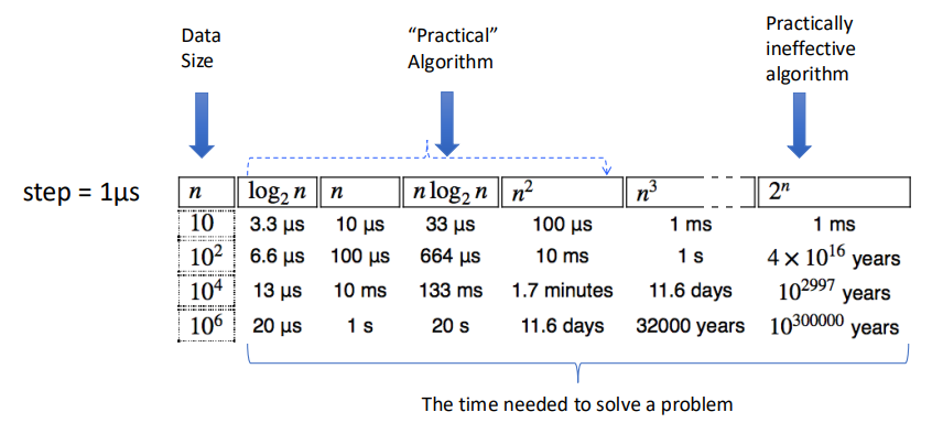
$T(n)$ is the largest (worst) execution time over all inputs of size $n$.
Asymptotic Complexity
Goal: Capture the growth of $T(n)$ of an algorithm as the problem instance size $n \rightarrow \infty$
Key Idea: Keep only the rate of growth, i.e., the dominant term when $n \rightarrow \infty$, forgetting multiplicative constants and lower order terms.
Three Os
-
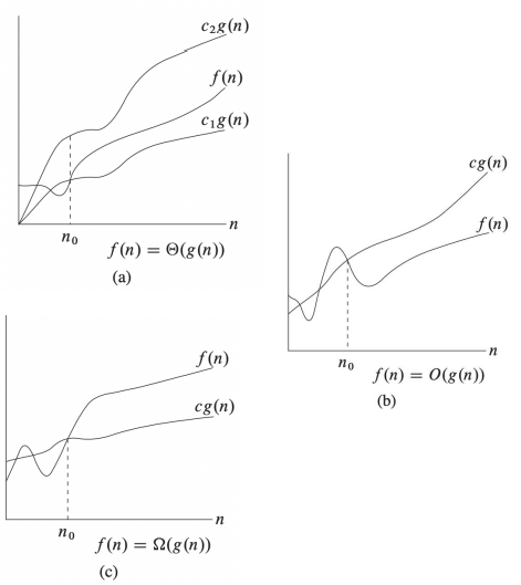
$\Theta$: Grows asymptotically as fast as ($=$)
- Tight Bound
- $f(n) = \Theta(g(n)) \Leftrightarrow \exists c_1, c_2 > 0, n_0 \text{ s.t. } c_1 g(n) \leq f(n) \leq c_2 g(n) \text{ for } n \geq n_0$
- e.g. $100n^2 + 5n - 5 = 0.1n^2 + 10n^{1.5} - 5 = \Theta(n^2)$
-
$O$: Grows asymptotically at most as fast as ($\leq$)
- Upper Bound
- $f(n) = O(g(n)) \Leftrightarrow \exists c > 0, n_0 \text{ s.t. } f(n) \leq c g(n) \text{ for } n \geq n_0$
- e.g. $2n^{1.5}-5 \leq n^{1.5} \leq n^2 \Rightarrow 2n^{1.5}-5 = O(n^{1.5}), = O(n^2)$
- e.g. $n^{1.5} \leq n^2 \leq 2^n \Rightarrow n^{1.5} = O(n^2), n^2 = O(2^n), n^{1.5} = O(2^n)$
-
$\Omega$: Grows asymptotically at least as fast as ($\geq$)
- Lower Bound
- $f(n) = \Omega(g(n)) \Leftrightarrow \exists c > 0, n_0 \text{ s.t. } f(n) \geq c g(n) \text{ for } n \geq n_0$
- e.g. $5 \leq 2n \leq n^{1.5}+1 \leq 2^n \Rightarrow 2n = \Omega(1), 2^n = \Omega(n^{1.5})$
In Practice
Conclusions
- To measure the performance of algorithms we measure their asymptotic complexity.
- Big $O$ is used to describe an upper bound for the running time of an algorithm.
- Big $\Omega$ is used to describe a lower bound for the running time of an algorithm.
- Big $\Theta$ is used to denote asymptotic equivalence of the running times of two algorithms. And when $\Omega(g(n)) = O(g(n)) = f(n)$, we can have $\Theta(g(n)) = f(n)$
L2 Divide and Conquer
Divide and Conquer (Sorting and Master Theorem)
Basic Devide and Conquer
There are 3 steps:
- Divide input into multiple smaller (usually disjoint) points.
- Conquer each of the parts separatelly (using recursive calls).
- Combine results from different calls.
$$ T(n) = \text{divide time} \\ +T(n_1) + T(n_2) + \cdots + T(n_k) \\ +\text{combine time} $$
Sorting
A non-D&C solution: Insertion Sort
void insertionSort(int arr[], int n) {
    for (int i = 1; i < n; i++) {
        int key = arr[i];
        int j = i - 1;
        while (j >= 0 && arr[j] > key) {
            arr[j + 1] = arr[j];
            j--;
        }
        arr[j + 1] = key;
    }
}
We have the complexity is $O(n^2)$ since it runs two loops with $n$ steps.
But $O(n^2)$ is too slow for most of the problem, can it be much faster? Of course. We can use divide and conquer here!
A D&C solution: Merge Sort
void merge(vector<int>& arr, int l, int m, int r) {
    int n1 = m - l + 1;
    int n2 = r - m;
    vector<int> L(n1), R(n2);
    for (int i = 0; i < n1; i++) L[i] = arr[l + i];
    for (int j = 0; j < n2; j++) R[j] = arr[m + 1 + j];
    int i = 0, j = 0, k = l;
    while (i < n1 && j < n2) {
        if (L[i] <= R[j]) arr[k++] = L[i++];
        else arr[k++] = R[j++];
    }
    while (i < n1) arr[k++] = L[i++];
    while (j < n2) arr[k++] = R[j++];
}

void mergeSort(vector<int>& arr, int l, int r) {
    if (l < r) {
        int m = l + (r - l) / 2;
        mergeSort(arr, l, m);
        mergeSort(arr, m + 1, r);
        merge(arr, l, m, r);
    }
}
From the function mergeSort we can see that we divide the array into $2$ parts and conquer them seperately and recursively. And the merge function has the time complexity of $\Theta(n)$.
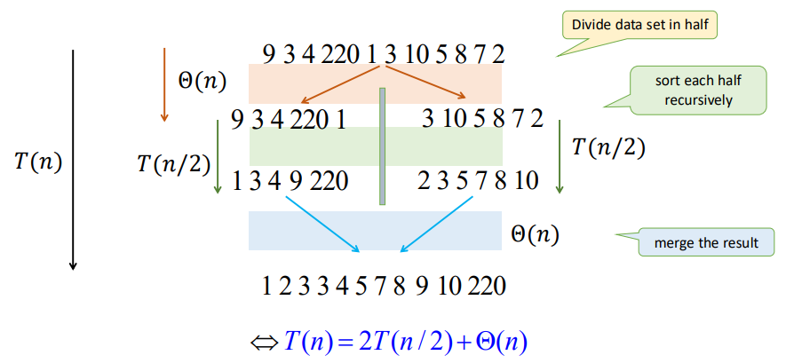
From the graph we can see that there is only $\log n$ levels of recursion. Thus, we have
$$ \begin{align*} T(n) &= 2T(n/2) + cn \\ &= (cn) \log n + nT(1) \\ &= \Theta (n \log n) \end{align*} $$
Where $cn$ denotes for the time of divide and merge, and $T(1)$ represents for the node of the recursion tree.
Geometric Sums
Consider a geometric series $$ S = 1 + x + x^2 + \cdots + x^h = \frac{x^{x+1}-1}{x-1} \ \ (\text{for } x \not= 1) $$ If $x < 1$, then $$ 1 + x + x^2 + \cdots + x^h \in \left[ 1, \frac{1}{1-x} \right] \Rightarrow S = \Theta(1) $$ If $x > 1$ , then $$ 1 + x + x^2 + \cdots + x^h < \frac{1}{1-x} x^h \Rightarrow S = \Theta(x^h) $$
Master Theorem
Consider the recursion:
$$ T(n) = aT(n/b) + f(n) $$
- Number of levels: $\log_b n = \Theta(\log n)$
- Number of leaves: $L = a^{\log_b n} = n^{log_b a}$
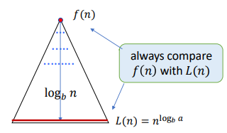
We use the recursion tree to calculate the cost. The cost of the $i$-th (root $i=0$) is: $$ \begin{align*} C_i &= (\text{Nodes Number of } i \text{-th Level}) \times (f \text{ of Every Subproblem}) \\ &= a^i f(n/b^i) \end{align*} $$ So that, we have: $$ T(n) = \sum_{i=0}^h C_i = \sum_{i=0}^{\log_b n} a^i f(n/b^i) $$
We need to compare the time within root and leaves to get the main factor. The usual method is to compare $f(n)$ and $L(n) = n^{\log_b a}$
There are 3 situations here:
-
Geometrically Increasing (Leaves): $$ f(n) = O(L^{1-\epsilon}) \Rightarrow T(n) = \Theta(L) $$ e.g. $T(n) = 2T(n/2) + \sqrt{n}$, we have $a=2, b=2, L=n^{\log_b a} = n$, and $\sqrt{n} = n^{1/2} = O(L^{1-\epsilon})$, thus $T(n) = \Theta(n)$
-
Roughly Equal Levels: $$ f(n) = \Theta(L) \Rightarrow T(n) = \Theta (L \log n) \\ f(n) = \Theta(L \log n) \Rightarrow T(n) = \Theta (L \log^2 n) $$ e.g. $T(n) = 2T(n/2) + n$, we have $L=n^{\log_2 2} = n$, and $n = O(L)$, thus $T(n) = \Theta(n \log n)$
-
Geometrically Decreasing (Root) + Regularly Condition $$ f(n) = \Omega(L^{1+\epsilon}) \text{ and } af(n/b) \leq sf(n), s < 1 \Rightarrow T(n) = \Theta(f(n)) $$ e.g. $T(n) = 2T(n/2) + n^2$, we have $L=n^{\log_2 2} = n$, and $n^2 > O(L), 2f(n/2) = 2(n/2)^2 \leq (1/2) f(n)$, thus $T(n) = \Theta(n^2)$
Applications of D&C
Convex Hull
Given $n$ points $S = { (x_i, y_i) | i = 1, 2, \cdots, n }$ s.t. all have different $x$ and $y$ coordinates, and no three of them in a line.
Convex Hull (CH): The smallest polygon containing all points in $S$. Represented by the sequence of points in the boundary in clockwise order.
How to use D&C here?
- Sort points by $x$-coordinate.
- For our input set $S$ of points:
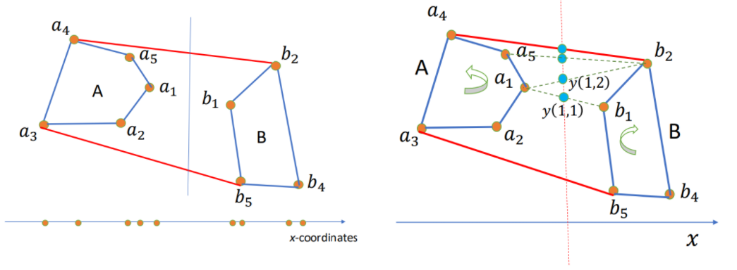
- Divide (by $x$-coordinates) into left-half A and right-half B.
- Compute CH(A) and CH(B).
- Merge CH(A) and CH(B) to get CH(A+B).
It has the complexity time $T(n) = 2T(n/2) + \Theta(n) \rightarrow \Theta(n \log n)$.
BUT, how to merge?
Algorithm: Start with $(a_1, b_1)$. While $y(i, j)$ increases, keep moving by one step either a_i counterclockwise or b_j clockwise. When cannot increase anymore, we found the upper tangent, say $a_u, b_u$. Similarly, the lower tangent $a_l, b_l$. Then the CH = points of A clockwise from $a_l$ to $a_u$ + points of B clockwise from $b_u$ + $b_l$. Hence total time $\Theta(n)$
Median Finding / Peak Finding
Not interested.
Fast Fourier Transform
Multiplication of polynomials as list of coefficients.
Consider: $$ \begin{align*} A(x) &= a_0 + a_1 x + \cdots + a_n x^n = \sum_{i=0}^{n}a_i x^i \\ B(x) &= b_0 + b_1 x + \cdots + b_n x^n = \sum_{i=0}^{n}b_i x^i \end{align*} $$ To calculate: $$ \begin{align*} C(x) &= A(x) B(x) = c_0 + c_1 x + \cdots + c_{2n}x^{2n} =\sum_{i=0}^{2n}c_i x^i \\ \text{where }c_k &= a_0 b_k + a_1 b_{k-1} + \cdots + a_k b_0 = \sum_{i=0}^k a_i b_{k-i} \end{align*} $$
Complexity: For $c_k \rightarrow O(k)$, for $C(x) \rightarrow O(n^2)$
Can we do it faster? Like $O(n \log n)$?
Multiplication of polynomials as list of values.
Consider: A degree-$n$ polynomial is uniquely characterized by its values at any $n+1$ distinct points $x_0, x_1, \cdots, x_d$.
That is, if we fix any distinct $n+1$ points, we can specify any degree-$n$ polynomial $A(x) = a_0 + a_1 x + \cdots + a_d x^n$ by the $n+1$ values: $$ A(x_0), A(x_1), \cdots, A(x_n) $$ Then we can have: $$ \begin{align*} C(x) &= A(x) B(x) \\ C(x_i) &= A(x_i) B(x_i) \\ \text{where } i&=0,1,\cdots,2n \end{align*} $$ Polynomial multiplication is $O(n)$ using this representation!
But how can we get the coefficients of $C(x)$ ?
Evaluation and Interpolation
Evaluation: $a_0, a_1, \cdots, a_n \rightarrow A(x_0), A(x_1), \cdots, A(x_n)$
$$ A(x) = M_n(x) \cdot a \\ $$ $$ \begin{bmatrix} A(x_0) \\ A(x_1) \\ \vdots \\ A(x_{n}) \end{bmatrix}= \begin{bmatrix} 1 & x_0 & x_0^2 & \cdots & x_0^n \\ 1 & x_1 & x_1^2 & \cdots & x_1^n \\ \vdots & \vdots & \vdots & \ddots & \vdots \\ 1 & x_n & x_n^2 & \cdots & x_n^n \end{bmatrix} \cdot \begin{bmatrix} a_0 \\ a_1 \\ \vdots \\ a_{n} \end{bmatrix} $$
Interpolation: $A(x_0), A(x_1), \cdots, A(x_n) \rightarrow a_0, a_1, \cdots, a_n$ $$ a = M_n^{-1}(x) \cdot A(x) \\ $$ $$ \begin{bmatrix} a_0 \\ a_1 \\ \vdots \\ a_n \end{bmatrix}= \begin{bmatrix} 1 & x_0 & x_0^2 & \cdots & x_0^n \\ 1 & x_1 & x_1^2 & \cdots & x_1^n \\ \vdots & \vdots & \vdots & \ddots & \vdots \\ 1 & x_n & x_n^2 & \cdots & x_n^n \end{bmatrix} ^{-1} \cdot \begin{bmatrix} A(x_0) \\ A(x_1) \\ \vdots \\ A(x_n) \end{bmatrix} $$
Here $M_n$ is Vandermonde matrix.
Consider $C(x_i) = A(x_i) B(x_i)$, from the two matrix multiplication we can know that: If we have every $A(x_i)$ and $B(x_i)$ we can use $O(n)$ to multiply and get $C(x_i)$, then transfer it into every coefficient $c_i$.
But, using matrix multiplication directly will need time complexity of $O(n^2)$. Can we optimize it to $O(n \log n)$? Yes, and here comes Fast Fourier Tranform (FFT).
FFT
Let's calculate evaluation using FFT first.
Consider a polynomial $P(x)$ with length of even number $n$ s.t. $$ \begin{align*} P(x) &= a_0 + a_1 x + a_2 x^2 + \cdots + a_{n-1} x^{n-1} \\ &= P_{\text{even}}(x^2) + x \cdot P_{\text{odd}}(x^2) \\ \text{where } P_{\text{even}}(x) &= a_0 + a_2 x + a_4 x^2 + \cdots + a_{n-2} x^{n/2} \\ P_{\text{odd}}(x) &= a_1 + a_3 x + a_5 x^2 + \cdots + a_{n-1} x^{n/2} \end{align*} $$
By doing this, we divide the the length $n$ to two length $n/2$. Then, we have to conquer them each and then combine them together.
Let $A_k$ denote $A(x_k)$.
The question is: How can we divide $A_k$?
And here's the most essencial part: We use primitive root $\omega$.
Now, think about an complex equation: $$ z^n = (re^{i\theta})^n = 1 $$ We can get the solutions: $$ \begin{align*} r &= 1 \\ \theta &= \frac{2k\pi}{n} \\ \text{where } k &= 0, 1, \cdots, n-1 \end{align*} $$ Thus, $$ \begin{align*} \omega_n &= e^{\frac{2\pi}{n}i} \\ \omega_n^k &= e^{\frac{2\pi}{n}ki} = e^{i\theta} \\ (\omega_n^k)^n &= 1 \end{align*} $$ To each $k$, we want to calculate: $$ \begin{align*} A_k &= P(\omega_n^k) \\ &= P_{\text{even}}(\omega_n^{2k}) + \omega_n^k \cdot P_{\text{odd}}(\omega_n^{2k}) \\ &= P_{\text{even}}(\omega_{n/2}^{k}) + \omega_n^k \cdot P_{\text{odd}}(\omega_{n/2}^{k}) \end{align*} $$ Since $$ \omega_n^{2k} = e^{\frac{2\pi}{n} 2ki} = e^{\frac{2\pi}{n/2} ki} = \omega_{n/2}^k $$ This is called the Discrete Fourier Tranform (DFT) of $A_k$.
And we found that: $$ \begin{align*} A_{k+n/2} &= P(\omega_n^{k+n/2}) \\ &= P_{\text{even}}(\omega_{n/2}^{k+n/2}) + \omega_n^{k+n/2} \cdot P_{\text{odd}}(\omega_{n/2}^{k+n/2}) \\ &= P_{\text{even}}(\omega_{n/2}^{k} \cdot \omega_{n/2}^{n/2}) + \omega_n^k \cdot \omega_n^{n/2} \cdot P_{\text{odd}}(\omega_{n/2}^{k} \cdot \omega_{n/2}^{n/2}) \\ &= P_{\text{even}}(\omega_{n/2}^{k}) - \omega_n^k \cdot P_{\text{odd}}(\omega_{n/2}^{k}) \end{align*} $$ Since $$ \omega_n^n = e^{\frac{2\pi}{n}ni} = e^{2\pi i} = 1 \\ \omega_n^{n/2} = e^{\frac{2\pi}{n} (n/2)i} = e^{\pi i} = -1 $$
Combining $A_k$ and $A_{k+n/2}$ together for $0 \leq k < n/2$, we can do D&C here! Since $P_{\text{even}}(\omega_{n/2}^{k})$ and $P_{\text{odd}}(\omega_{n/2}^{k})$ can calculate from the half DFT.
The time complexity is $T(n) = 2T(n/2) + O(n) = O(n \log n)$. We get the whole evaluation.
IFFT
To do interpolation, we need Inverse Fast Fourier Tranfrom (IFFT).
Inverse FFT is easy to explain using Linear Algebra.
It's easy since: $$ a = M_n^{-1}(\omega) \cdot A(\omega) = \frac{1}{n} M_n(\omega^{-1}) \cdot A(\omega) $$ And it's over.
Let $A(\omega) = \text{FFT}(a, \omega)$, then $a = \frac{1}{n} \text{FFT}(A, \omega^{-1})$.
The Whole Progress
- Filled $A(x)$ and $B(x)$ to length of $n=2^k$ by $0$ due to easier FFT D&C.
- Calculate $A(\omega^k)$ and $B(\omega^k)$ for each $k=0,1,\cdots,n-1$, where $\omega = e^{\frac{2\pi}{n}i}$ using FFT.
- Calculate $C(\omega^k) = A(\omega^k) \cdot B(\omega^k)$.
- Calculate $c_i$ using IFFT.
L3 Randomized Algorithms
Basic Concepts of Randomized Algoirthms
Randomized Algorithms: On the same input, different executions of the same algorithm may result in different running times and different outputs.
Type of polynomial randomized algorithms:
- Monte Carlo: Bounded number of steps, but might not find the answer.
- Runs in polynomial time, $P_r$(answer is correct)$=p_o > \frac{1}{2}$.
- Always able to check the answer for correctness.
- How to use: Repeat if neccessary, use majority of answers.
- Las Vegas: No guarantee on max number of steps, always finds answer.
- Runs in expected polynomial time.
- Not stop until finds the correct answer.
$\overline{T}(n)$: Expected time to terminate for a given input of size $n$.
Quicksort
Consider combining D&C and randomize
- Pick an pivot $x$ of the array.
- Divide: Partition the array into subarrays using $x$.
- Conquer: Recursively sort $A$, $B$.
- Combine: $A$, $x$, $B$.
$\overline{T}(n) = \Theta(n \log n)$ for all inputs. $\Rightarrow$ Random selection of $x$ makes no input to be worse.
Or we can say $\Theta(n \log n)$ is the average complexity of quicksort.
Frievald's Algorithm
Given $n \times n$ matrices $A$, $B$ and $C$, check that $AB = C$ (yes or no).
It's very slow to use brute force algorithm since matrices multiplication is $O(n^3)$.
Consider randomization (Frievald's Algorithm):
- Choose a random binary vector $r$.
- If $(A(Br) = Cr) \bmod 2$ then output "yes" else "no".
Property: If $AB \not= C$, then $\text{Pr}[A(Br) \not= Cr] \geq \frac{1}{2}$.
That is, Do 10 tests, if all say "yes", the probability of error $< \left( \frac{1}{2} \right)^{10}$.
L4 Lower Bounds and Heaps
Comparison Model
Comparsion Sort
All the sorting algorithms we've seen so far are comparison sort (merge sort, insertion sort, bubble sort, etc.).
And the best running time that we've seen for comparison sort is $O(n \log n)$. Is it the best we can do?
Decision-Tree
A given recipe for sorting $n$ numbers $a_1, a_2, \cdots, a_n$.
Nodes are suggested comparisons: $i, j$ means compare $a_i$ to $a_j$ for $i, j \in \{1, 2, \cdots, n\}$
The figure below is an example of decision-tree of sorting $a_1 = 9, a_2 = 4, a_3 = 6$.
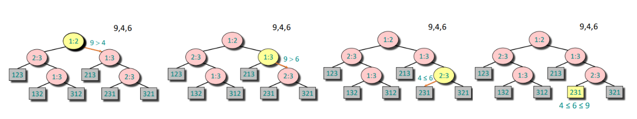
From the tree we can see that:
- A path from the root to the leaves of the tree represents a trace of comparisons that the algorithm may perform.
- The running time of the algorithm = the length of the path taken.
- Worst-case running time = height(depth) of tree
The tree must contain $\geq n!$ leaves since there are $n!$ possible permutations. And a height-$h$ binary tree has $L_h \leq 2^h$ leaves.
Hence: $$ n! \leq L_h \leq 2^h \iff h > \log(n!) \iff h = \Omega(n \log n) $$
Since the Stirling's approximation: $$ n! \approx \sqrt{2 \pi n} \left(\frac{n}{e}\right)^n \\ \log(n!) = n \log n - n + \frac{1}{2} \log (2 \pi n) $$
Theorem: Any decision tree that can sort $n$ elements must have height $\Omega(n \log n)$.
Linear Time Sorting
As metioned above, the comparison sorting have a lower-bound complexity of $\Omega(n \log n)$, so do linear time sorting exist?
Counting Sort
Given: An array $a_0, a_1, \cdots, a_{n-1}$ of $n$ keys to be sorted.
Count the times of number appeared between $a_{min}$ and $a_{max}$, then use the prefix sum array to get the final place of each element. With time complexity of $O(n+k), k = a_{max} - a_{min} + 1$
void counting_sort(vector<int>& a) {
    int n = a.size();
    int mn = *min_element(a.begin(), a.end());
    int mx = *max_element(a.begin(), a.end());
    int k = mx - mn + 1;
    vector<int> count(k, 0);
    for (int x : a) count[x - mn]++;
    for (int i = 1; i < k; i++) count[i] += count[i - 1];
    vector<int> res(n);
    for (int i = n - 1; i >= 0; i--) {
        int x = a[i];
        res[--count[x - mn]] = x;
    }
    a = res;
}
Radix Sort
Use a radix(base) $k$ for an integer $x$: $$ x = a_{d-1} k^{d-1} + \cdots + a_0 k^0 \to a_{d-1}a_{d-2}\cdots a_0 $$
Idea: Sort on least-significant digit first with auxiliary stable sort.
We are given $n$ integers, each integer $< M$, in base $k$. Then we have time complexity of $O((n+k) \log_k M)d$
Heaps
Storing Objects in Data Structures
We operate on objects of the form: object $x = (x.\text{key}, x.\text{data})$.
The attribute $x.\text{key}$ characterizes uniquely the object $x$. And we store $x.\text{key}$ combined with a pointer to the location of $x.\text{data}$ in memory.
Inserting and searching for object $x$ is done by inserting and searching for $x.\text{key}$. Or we can say we mostly focus on $x.\text{key}$ instead of $x.\text{data}$.
Priority Queue
$S$: set of elements $\{ x_1, x_2, \cdots, x_n \}$.
$x_i = (\text{key}_i, \text{data}_i)$.
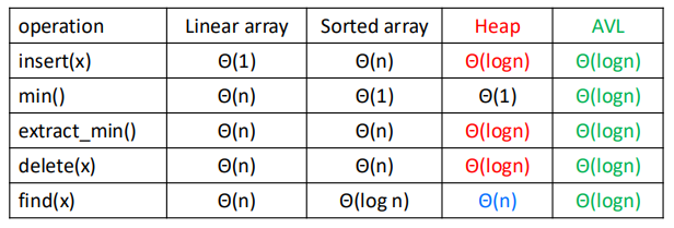
Operations: $\text{Insert}(S,x), \max(S), \text{Extract-max}(S), \text{Incr-key}(S, x, k)$.
Heap
Heap: An array visualized as a nearly complete binary tree.
Navigate on the tree but move on array = full info of the tree, without pointers.
Max(Min) Heap Property: the key of a node is $\geq (\leq)$ than the keys of its children.
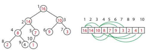
Binary Tree Structure in array, as shown above.
int s[MAXN], sz;

int parent(int i) {
    return i >> 1; // i/2
}

int left(int i) {
    return i << 1; // i*2
}

int right(int i) {
    return i << 1 | 1; // i*2+1
}
And the height of the tree is $h = \log n$.
Max Heapify: Correct a single violation of the heap property occurring at the root $i$ of a subtree in $O(\log n)$.
void max_heapify(int i) {
    int l = left(i), r = right(i), maxi = i;
    if(l <= sz && s[l] > s[maxi]) maxi = l;
    if(r <= sz && s[r] > s[maxi]) maxi = r;
    if(maxi != i) {
        swap(s[i], s[maxi]);
        max_heapify(maxi);
    }
}
Build Max Heap: Convert an array $A$ into a max heap. And we find that elements from $A_{\lfloor n/2 \rfloor+1}$ to $A_n$ are leaves of the tree, and they won't violate the rule. So we only need to heapify $A_1$ to $A_{\lfloor n/2 \rfloor}$. The time complexity is $O(n)$.
void build_max_heap(int n) {
    sz = n;
    for(int i = n/2; i >= 1; i--) max_heapify(i);
}
Insert: We first put it at the back of the array, then go up in the tree one level by one level until no violation.
void insert(int val) {
    sz++;
    s[sz] = val;
    int i = sz;
    while(i > 1 && s[parent(i)] < s[i]) {
        swap(s[i], s[parent(i)]);
        i = parent(i);
    }
}
Extract Max: The max element must be the first one of the array, we can just swap it with the last element, then heapify.
int extract_max() {
    if(!sz) return -1;
    int maxn = s[1];
    s[1] = s[sz];
    sz--;
    max_heapify(1);
    return maxn;
}
Heap Sort: Like extracting max element for $n$ times. Time complexity $O(n \log n)$.
void heap_sort() {
    int n = sz;
    for(int i = n; i >= 2; i--) {
        swap(s[1], s[i]);
        sz--;
        max_heapify(1);
    }
}
L5 Trees
Binary Search Tree
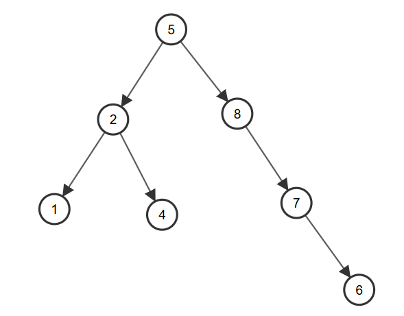
A Binary Search Tree(BST) is a binary tree structure that every node $x$ of it must satisfies:
- All $\text{key}$ from its left subtree is less than $x.\text{key}$
- All $\text{key}$ from its right subtree is greater than $x.\text{key}$
And we can easily know that the left subtree and right subtree of $x$ are both BST.
Define Node: Using C++ struct and pointers.
struct node {
    int key;
    node* left;
    node* right;
    node(int k): key(k), left(NULL), right(NULL) {}
};
Insert: Start from the root, if the $\text{key}$ is less, put it to the left, else to the right. Doing the whole progress in recursion, until find an empty place and put it in. With average time complexity $O(\log n)$, but worst $O(n)$.
node* insert(node* root, int key) {
    if(!root) return new node(key);
    if(key < root->key) {
        root->left = insert(root->left, key);
    } else if(key > root->key) {
        root->right = insert(root->right, key);
    }
    return root;
}
Build Tree: Actually there's no such a thing, you just need to insert the new node into root.
node* root = NULL;
root = insert(root, a);
Inorder Traversal: The inorder traversal of the BST is a sorted array, due to the property of it.
void printTree(node* root) {
    if(!root) return;
    printTree(root->left);
    cout << root->key << " ";
    printTree(root->right);
}
Search: Tipical binary search on tree.
node* search(node* root, int key) {
    if(!root || root->key == key) {
        return root;
    }
    if(key < root->key) {
        return search(root->left, key);
    } else {
        return search(root->right, key);
    }
}
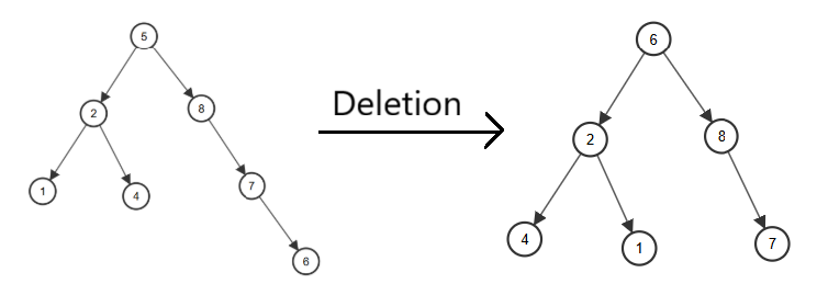
Delete: A bit complicated.
- Leaf (no children): Delete directly.
- On child: Use the child to replace it.
- Two children: Find the minimum of right subtree, replace it with the element we want to delete, and delete it.
node* deleteNode(node* root, int key) {
    if(!root) return NULL;

    if(key < root->key)
        root->left = deleteNode(root->left, key);
    else if(key > root->key)
        root->right = deleteNode(root->right, key);
    else {
        if(!root->left && !root->right) {
            delete root;
            return NULL;
        } else if(!root->left) {
            node* temp = root->right;
            delete root;
            return temp;
        } else if(!root->right) {
            node* temp = root->left;
            delete root;
            return temp;
        } else {
            node* temp = findMin(root->right);
            root->key = temp->key;
            root->right = deleteNode(root->right, temp->key);
        }
    }
    return root;
}
Warning: We usually use the different key to insert, but if there exists two same keys, we can do a count, or change the right subtree to greater or equal subtree.
AVL Tree
An AVL (Adelson-Velskii and Landis) Tree is a self-balancing binary search tree.
Property: For every node, store its height:
- Leaves have height $0$
- NIL has height $-1$
Invariant: For every node $x$, the heights of its left child and right child differ by at most $1$.
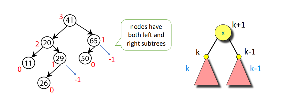
And we can know that AVL trees always have height $\Theta(\log n)$.
Define Node: Like BST, but with height.
struct node {
    int key, height;
    node* left;
    node* right;
    node(int k): key(k), height(1), left(NULL), right(NULL) {}
};
Get Height: For convenience, I take leaves height as $1$, NIL height as $0$.
int getHeight(node* u) {
    return u ? u->height : 0;
}
Get Balance: Use the definition of balance, $\text{BL} = \text{height}(\text{left subtree}) - \text{height}(\text{right subtree})$, notice that if $\text{BL} > 1$, left subtree is heavy, else if $\text{BL} < 1$, right subtree is heavy, else it's balanced at this node.
int getBalance(node* u) {
    return u ? getHeight(u->left) - getHeight(u->right) : 0;
}
Right Rotate:
      A                 B
     / \               / \
    B   T3    ->      T1  A
   / \                   / \
  T1  T2                T2  T3
node* rightRotate(node* u) {
    node* v = u->left;
    node* w = v->right;
    v->right = u;
    u->left = w;
    u->height = max(getHeight(u->left), getHeight(u->right)) + 1;
    v->height = max(getHeight(v->left), getHeight(v->right)) + 1;
    return v;
}
Left Rotate:
    A                      B
   / \                    / \
  T1  B        ->        A   T3
     / \                / \
    T2  T3             T1  T2
node* leftRotate(node* u) {
    node* v = u->right;
    node* w = v->left;
    v->left = u;
    u->right = w;
    u->height = max(getHeight(u->left), getHeight(u->right)) + 1;
    v->height = max(getHeight(v->left), getHeight(v->right)) + 1;
    return v;
}
Insert: Consider insertion with 4 situations (L and R means insert into left and right subtree):
- LL: Do right rotation once.
- RR: Do left rotation once.
- LR: Do left rotation, then right rotation.
- RL: Do right rotation, then left rotation.
node *insert(node* u, int key) {
    if(!u) return new node(key);
    if(key < u->key) u->left = insert(u->left, key);
    else if(key > u->key) u->right = insert(u->right, key);
    else return u;
    u->height = max(getHeight(u->left), getHeight(u->right)) + 1;
    int BL = getBalance(u);
    if(BL > 1 && key < u->left->key) return rightRotate(u); // LL
    if(BL < -1 && key > u->right->key) return leftRotate(u); // RR
    if(BL > 1 && key > u->left->key) { // LR
        u->left = leftRotate(u->left);
        return rightRotate(u);
    }
    if(BL < -1 && key < u->right->key) { // RL
        u->right = rightRotate(u->right);
        return leftRotate(u);
    }
    return u;
}

Delete: As same as deletion in BST, then check whether it's balanced.
node* findMin(node* u) {
    while(u->left) u = u->left;
    return u;
}

node* deleteNode(node* u, int key) {
    // BST Deletion first
    if(!u) return NULL;
    if(key < u->key) u->left = deleteNode(u->left, key);
    else if(key > u->key) u->right = deleteNode(u->right, key);
    else {
        if(!u->left || !u->right) {
            node* temp = u->left ? u->left : u->right;
            if(!temp) {
                temp = u;
                u = NULL;
            } else {
                *u = *temp;
            }
            delete temp;
        } else {
            node* temp = findMin(u->right);
            u->key = temp->key;
            u->right = deleteNode(u->right, temp->key);
        }
    }
    if(!u) return NULL;
    // Keep balance
    u->height = max(getHeight(u->left), getHeight(u->right)) + 1;
    int BL = getBalance(u);
    if(BL > 1 && getBalance(u->left) >= 0)
        return rightRotate(u); // LL
    if(BL > 1 && getBalance(u->left) < 0) {
        u->left = leftRotate(u->left);
        return rightRotate(u); // LR
    }
    if(BL < -1 && getBalance(u->right) <= 0)
        return leftRotate(u); // RR
    if(BL < -1 && getBalance(u->right) > 0) {
        u->right = rightRotate(u->right);
        return leftRotate(u); // RL
    }
    return u;
}
Time Complexity: In balanced BST, all operations take $O(\log n)$.
Red-Black Tree
Shit.
Interval Tree
Interval Tree is a balanced BST but nodes are intervals.
Define Node: Interval has $l$ and $r$, while $\text{maxn}$ is the maximum $r$ of all interval of the whole subtree, and we use $l$ as the $\text{key}$ of BST.
struct interval {
    int l, r;
};

struct node {
    interval i;
    int maxn;
    node* left;
    node* right;
    node(interval in): i(in), maxn(in.r), left(NULL), right(NULL) {}
};
Insert: Like regular BST, using $l$ as the $\text{key}$, and record $\text{maxn}$.
node* insert(node* u, interval i) {
    if(!u) return new node(i);
    if(i.l < u->i.l) u->left = insert(u->left, i);
    else u->right = insert(u->right, i);
    u->maxn = max(u->maxn, i.r);
    return u;
}
Search: To get all the intervals who are overlapping with $i$, there are 3 situations
- If the node has overlap with $i$, record the answer.
- If its left subtree's $\text{maxn}$ is greater than $i.l$, search in the left subtree.
- If the node's $l$ is less than $i.r$, search in the right subtree.
bool isOverlap(interval a, interval b) {
    return a.l <= b.r && a.r >= b.l;
}

void searchAll(node* u, interval i, vector<interval>& re) {
    if(!u) return;
    if(isOverlap(u->i, i)) re.push_back(u->i);
    if(u->left && u->left->maxn >= i.l) searchAll(u->left, i, re);
    if(u->right && u->i.l <= i.r) searchAll(u->right, i, re);
}
The regular Interval Tree is like BST with worst time complexity $O(n)$ for each operation, but it can be optimized by AVL tree or other balanced tree, reducing the time complexity to $O(\log n)$.
vEB Tree
An vEB (van Emde Boas) Tree is a data structure that can support below functions in a integer set $S \subseteq \{ 0, 1, \cdots, U-1 \}$, while $U$ is the range of integers (e.g. $U=2^{16}$)
L6 Hashing
Basic Concepts of Hashing
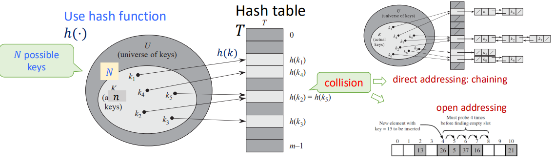
Hash Function: A function that maps data of arbitrary size to fixed-sized values. And the goal is to propose a data structure such that for key $k$:
- $\text{add}(k), \text{delete}(k) = O(1)$
- $\text{search}(k) = O(1)$ on the average
From what I've learnt, the most important thing is not the precise hashing function itself, but the critical thought of hashing.
Hash Table: A table that stores indice and values of hashing.
Making Choices
Choosing the Keys:
- By Nature: Randomly from $U$. (Simple uniform hashing)
- By an Opponent: That knows the hash function we use when this is fixed, in a way to create the longest possbile chain. (Universal hashing)
Choosing the Hash Funcions:
- We use a fixed hash function everyone knows.
- We change before each experiments the hash function, chosen randomly from a "universal set" of functions known to everyone.
Special Case (perfect hashing): We know the keys, then choose the hash function.
Performance: Average length of chain in a typical slot (same hashing value).
Models for Randomness
Simple Uniform Hashing Assumption (SUHA)
$h$ is fixed: In every experiment each key $k$'s value is chosen randomly (uniformly) from $U$.
- Then, $h$ is "good" if $h(k)$ scatters uniformly over the hash table: $$ P_k[h(k) = i] = \frac{1}{m}, \forall i = 1, 2, \cdots, m $$
- We call this the Simple Uniform Hashing Assumption.
Universal Hashing
The set of keys to be stored is assumed fixed: In every experiment, $h$ is randomly (uniformly) chosen from a set $H$.
- Then, $H$ is "good" if $$ P_h[h(k_1) = h(k_2)] \leq \frac{1}{m}, \forall k_1 \not= k_2 $$
- $H$ is a set of Universal Hash Funcions
Actually, Universal Hashing is not a hash function, but designing a set of hash functions. It will randomly choose a hash function when using. Or we can san Universal Hashing is using SUHA by randomization, in order to decrese the probability of collisions.
Universal Hashing Function Examples
The Matrix Method
Settings:
- Keys are $u$-bits long, $|U| = 2^u$
- Hash values are $b$-bits long, hash table size $m = 2^b$
And we pick $h = $ random $b \times u$ $0/1$ matrix, define: $$ h(x) = h \cdot x \pmod 2 $$
Which means matrix multiplication under module $2$.
Claim: For $x \not= y, P_h[h(x) = h(y)] \leq \frac{1}{m} = \frac{1}{2^b}$
e.g. $$ x = 2 = \begin{bmatrix} 1 \\ 0 \\ 1 \\ 0 \end{bmatrix}, h = \begin{bmatrix} 1 & 0 & 0 & 0 \\ 0 & 1 & 1 & 1 \\ 1 & 1 & 1 & 0 \end{bmatrix} $$ And we get $$ h(x) = h \cdot x = \begin{bmatrix} 1 \\ 1 \\ 0 \end{bmatrix} = 6 $$
Linear Hashing for Vector Keys
Settings:
- Suppose keys are vectors $x = (x_1, x_2, x_3, x_4)$, where $x_i$ is an $8$-bit integer. (i.e. $0 \leq x \leq 255$)
- We use a hash table of size $m = p$, where $p$ is a prime number slightly greater than $255$ (e.g. $257$).
Choose the vector of coefficients $a = (a_1, a_2, a_3, a_4)$ where $a_i$ is (uniformly) randomly selected in the range $\{0, 1, \cdots, m-1\}$ And we define: $$ h_a(x) = \left( \sum_{i=1}^4 a_i x_i \right) \bmod m $$
So the hash family is $$ H = \{ h_a : a \in [0, m-1]^4 \} $$
Claim: For $x \not= y, P_a[h_a(x) = h_a(y)] = \frac{1}{m}$
Affine Hashing for Integer Keys
Also called the Carter-Wegman construction
Settings:
- Keys are integers $k \in U$
- Pick a prime number $p$ s.t. $|U| \leq p \leq 2|U|$
- Table size $m \leq p$
We radomly choose $a \in \{ 1, 2, \cdots, p-1 \}, b \in \{ 0, 1, \cdots, p-1 \}$, and define: $$ h_{a,b}(k) = ((a \cdot k + b) \bmod p) \bmod m $$
Claim: For $x \not= y, P_{a,b}[h_{a,b}(x) = h_{a,b}(y)] \leq \frac{1}{m}$
e.g. $|U| = 2^4 = 16, p = 17, m = 6, k = 8, a = 3, b = 4$, then: $$ h_{3,4}(8) = ((3 \cdot 8 + 4) \bmod 17) \bmod 6 = 5 $$
Rolling Hash
Sliding window, but in hashing.
Rabin-Karp Algorithm
Consider a string $S = s_0 s_1 s_2 \cdots s_{n-1}$. We define a window of length $k$ s.t. $T = s_i s_{i+1} \cdots s_{i+k-1}$. And we use the polynomial hash function: $$ H_i = H(T) = (s_i \cdot p^{k-1} + s_{i+1} p^{k-2} + \cdots + s_{i+k-1} \cdot p^0) \bmod M $$ Where $p$ is the base, $M$ is a large prime number and $s_i$ is the ASCII number.
From the function above we can get: $$ H_{i+1} = ((H_i - s_i \cdot p^{k-1}) \cdot p + s_{i+k}) \bmod M $$
And then we can $O(1)$ check whether a string of length $k$ is appeared in $S$.
Table Doubling
We define Load Factor: $$ \alpha = \frac{n}{m} $$ Where $n$ is the element number in hash table, $m$ is the bucket number of hash table.
We have known that we need a hash table to store the keys and values, but if the element number in table is too large, it will cause more and more collisions, which slowing down the hashing progress.
So if $\alpha$ is too large (usually $1$), we will double the bucket number $m$, then rehash all the elements into new table.
Average Cost of Insertions $=\frac{2^{i+2}c + 2^i c_0}{2^i} = O(1)$
Or observe that up to any time $t$: by paying $O(1)$ per insert, covers at all times the total actual cost. We say that insert has an amortized cost of $O(1)$.
Perfect Hashing
Bloom Filters
L7 Amortized Analysis
Why Amortized Complexity?
Think about doubling hash tables, some of the functions are cheap, like $O(1)$ calculate hashing, but some are expensive, like $O(n)$ to doubling hash tables.
Amortized analysis is a way to make sure each function is in an average time, no need to assume randomized input.
Actual Cost and Amortized Cost
$c(t) = $ actual cost of the operation at time $t$. It can be a function of the state of the data structure, e.g. depends on $n$ = number of elements stored at time $t$.
$a(t) = $ amortized cost of the operation at time $t$. Assume $a(t) = O(1) \ \forall t$, i.e., $a(t) \leq c_a \ \forall t$
Suppose that we have shown that on any trajectory $0, 1, \cdots, T$, $$ \sum_{0 \leq t \leq T} c(t) \leq \sum_{0 \leq t \leq T} a(t) $$
Which means at any operation, the total actual cost $\leq$ the total budget cost we assigned. That is, our budget is enough to cover all the cost.
For any length $T$, $$ \sum_{0 \leq t \leq T} c(t) \leq \sum_{0 \leq t \leq T} a(t) \leq c_a T $$
Amortization Methods
Aggregate Method
The easiest way of amortization.
$$ \text{amortized cost per op} = \frac{\text{total cost of } k \text{ ops}}{k} $$
Amortized Bound
Define an amortized cost $a_op(t) = O(1)$ to each operation type s.t. for any possible sequence of operations, the total cost is covered. That is, $$ \sum(\text{amortized costs}) \geq \sum(\text{actual costs}) $$
Methods: Accounting method, Charging method, Potential method.
L8 Graphs
Graph Definition
$G = (V, E)$
$V$: A set of vertices. $|V|$ usually denoted by $n$.
$E \subseteq V \times V$: A set of edges (pair of vertices). $|E|$ usually denoted by $m$.
$m \leq n^2 = O(n^2)$
Two flavors:
- Directed graph: Edges have order.
- Undirected graph: Ignore order. Then only $\frac{n(n-1)}{2}$ possible edges.
Problems Relates to Graphs
Reachability: Find all states reachable from a given state.
Shortest Paths: Find the shortest path between state $s_0$ and $s_d$.
Cycle: Find if a directed graph has a cycle.
Topological Sort: Find a causal ordering of the nodes if it exists.
Minimum Spanning Tree: Find the minimum subgraph that contains all nodes.
Strongly Connected Components: Maximal sets of nodes that from every node can reach any other node in the set (mixing).
Graph Representation
Four representations with pros/cons:
- Adjacency Lists (of neighbors for each vertex)
- Incidence Lists (of edges from each vertex)
- Adjacency Matrix (0-1, which pairs are adjacent)
- Implicit representation (as a find neighbor function)
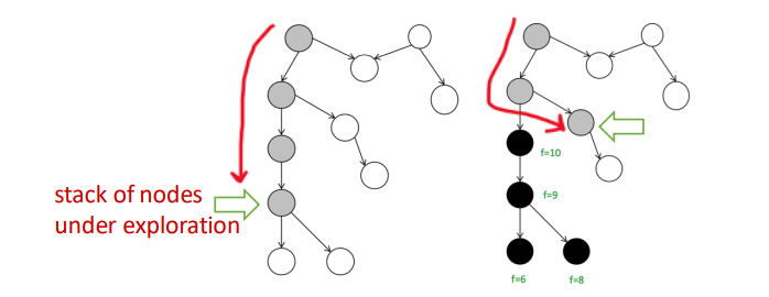
DFS
Depth-First Search (DFS) is a versatile linear-time procedure that reveals a wealth of information about a graph.
int n, m;
vector <int> g[MAXN];
int vis[MAXN]; // 0: WHITE, 1: GREY, 2: BLACK
int d[MAXN], f[MAXN], cnt;

void dfs(int u) {
    cnt++;
    d[u] = cnt;
    vis[u] = 1;
    for(int x = 0; x < g[u].size(); x++) {
        int v = g[u][x];
        if(!vis[v]) dfs(v);
        if(vis[v] == 1) cout << "Cycle!" << endl;
    }
    cnt++;
    f[u] = cnt;
    vis[u] = 2;
}
Properties of DFS
When DFS a graph, we will record two time stamp of each vertex:
- $d[u]$: Discover Time, when $u$ is first visited.
- $f[u]$: Finish Time, when we finish exploring all neighbors of $u$.
Of course, it's easy to see that $u.d < u.f$
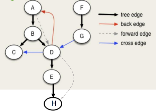
Then we can get $4$ different type of edges, for a $u \to v$:
- Tree Edge: When we first discover a new vertex $v$ from $u$.
- $u.d < v.d < v.f < u.f$
- Back Edge: An edge that points back to an ancestor in the DFS tree.
- $v.d < u.d < u.f < v.f$
- Forward Edge: An edge that goes from a node to its descendant in the DFS tree, but not a direct tree edge.
- $u.d < v.d < v.f < u.f$
- Cross Edge: An edge that goes between two different DFS branches (neither ancestor nor descendant).
- $v.d < v.f < u.d < u.f$
White Path Theorem
We colored the vertex in DFS:
- White: Not yet visited
- Gray: Currently being explored
- Black: Finished exploring
If, during a DFS, there is a path from a vertex $u$ to a vertex $v$ that only goes through white vertices, then $v$ will become a descendant of $u$ in the DFS tree.
We can use it to detect cycle in graph: When we see a back edge, or meet grey node, means we found a path from a node $u$ back to one of its ancestors $v$, and there is a cycle.
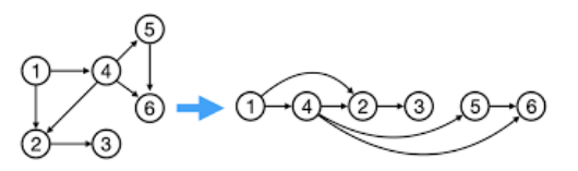
Topological Sort
Topological Sort of a DAG $G=(V,E)$.
Theorem: $G$ is a DAG iff there is a linear ordering of all its $v \in V$ s.t., if $(u, v) \in E$, then $u < v$ in the above ordering. Or we say $(u,v)$ goes always from left to right.
Algorithm: Given DAG $G$.
- Run any DFS($G$), compute finishing time of nodes.
- Linear order: The nodes in decreasing order of finishing times.
Corollary: In a DAG, $(u, v) \in E \iff u.f > v.f$ for any DFS.
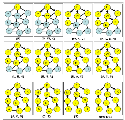
BFS
Breath-First Search (BFS) is searching neighbors around each node. And we usually use queue to implement.
Used very often in Shortest Path Algorithms.
int n, m;
vector <int> g[MAXN];
bool vis[MAXN];

void bfs(int st) {
    queue <int> q;
    q.push(st);
    vis[st] = true;
    while(!q.empty()) {
        int u = q.front(); q.pop();
        for(int x = 0; x < g[u].size(); x++) {
            int v = g[u][x];
            if(!vis[v]) {
                vis[v] = true;
                q.push(v);
            }
        }
    }
}
SCC
Strongly Connected Component (SCC): Maximal set of vertices $C \subseteq V$ such that for every pair of vertices $u, v \in C$, we have both $u \leadsto v$ and $v \leadsto u$.
$u \leadsto v$ means there is a path from $u$ to $v$.
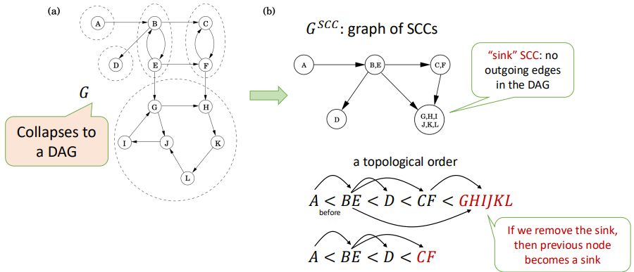
Kosaraju's Algorithm
Goal: Find all SCCs.
Key Observation: If you collapse each SCC into a single node, the resulting graph is a DAG. This DAG has a topological order.
If you start a DFS on a node located in a sink SCC (an SCC with no outgoing edges in the SCC DAG), the DFS will visit all nodes within that SCC and then stop, without leaking into other SCCs. You could then remove this SCC and repeat the process.
Idea: Reverse the direction of all edges in $G$ to create the transpose graph $G^T$.
int n, m;
vector<int> g[MAXN];      // original graph
vector<int> gr[MAXN];     // reversed graph
int vis[MAXN];
int d[MAXN], f[MAXN], cnt;
vector<int> order;        // store vertices by finish time
vector<int> component;    // store one SCC

void dfs1(int u) {
    vis[u] = 1;
    cnt++;
    d[u] = cnt;
    for (int v : g[u]) {
        if (!vis[v])
            dfs1(v);
    }
    cnt++;
    f[u] = cnt;
    order.push_back(u); // store vertex by finish time
    vis[u] = 2;
}

void dfs2(int u) {
    vis[u] = 1;
    component.push_back(u);
    for (int v : gr[u]) {
        if (!vis[v])
            dfs2(v);
    }
}

// Kosaraju main
void kosaraju() {
    cnt = 0;
    memset(vis, 0, sizeof(vis));
    for (int i = 1; i <= n; i++) {
        if (!vis[i])
            dfs1(i);
    }
    memset(vis, 0, sizeof(vis));
    reverse(order.begin(), order.end());
    cout << "Strongly Connected Components:\n";
    for (int u : order) {
        if (!vis[u]) {
            component.clear();
            dfs2(u);
            for (int x : component) cout << x << " ";
            cout << "\n";
        }
    }
}
And we can find all the SCCs using 2 DFS, with time complexity $O(n + m)$.
After Midterm (1 DAY BEFORE FINAL)
妈的,没时间了,得赶紧速通了
最短路(单源)
对于一个图 $G(V,E)$,其中两点 $u, v \in V$ 的最短路长度定义为 $\delta(u, v)$,且容易得到: $$ \delta(s, t) \leq \delta(s, u) + \delta(u, t) $$
Bellman-Ford
核心思想:对所有边执行 $n-1$ 轮松弛,复杂度 $O(nm)$
struct Edge {
    int u, v;
    LL w;
};

vector<Edge> edges;
vector<LL> dist;
int n, m, s;

bool bellman_ford() {
    dist.assign(n + 1, LLONG_MAX);
    dist[s] = 0;

    // n-1 次松弛
    for (int i = 1; i <= n - 1; i++) {
        bool updated = false;
        for (auto &e : edges) {
            if (dist[e.u] != LLONG_MAX &&
                dist[e.u] + e.w < dist[e.v]) {
                dist[e.v] = dist[e.u] + e.w;
                updated = true;
            }
        }
        if (!updated) break; // 提前结束
    }

    // 第 n 次检查负环
    for (auto &e : edges) {
        if (dist[e.u] != LLONG_MAX &&
            dist[e.u] + e.w < dist[e.v]) {
            return false; // 有负环
        }
    }
    return true; // 无负环
}
Dijkstra
核心思想:每一步都“贪心”地确定一个当前距离最小的点,并且一旦确定,就不会被更改。
算法维护两个集合:一个 $S$ 表示最短路已经被确定的点,还有一个 $V-S$ 表示还没被确定的点。每一步做三件事:
- 在 $V-S$ 中找到 $d$ 最小的点 $u$
- 把 $u$ 加入 $S$
- 用 $u$ 去松弛所有出边
那么,这个 $u$ 总是当前离 $s$ 最近的未确定点,不可能被绕路更短。
注意:没有负权的情况下
struct node {
	int v, dis;
};

struct pri {
	int ans, id;
	bool operator < (const pri &x) const{return x.ans < ans;}
};

priority_queue <pri> q;
vector <node> g[MAXN];
int n, m, d[MAXN], pre[MAXN];
bool vis[MAXN];

void Dijkstra(int st) {
	for(int x = 1; x <= n; x++) {
        d[x] = INF;
        pre[x] = -1;
        vis[x] = false;
    }
	d[st] = 0;
	q.push((pri){0, st});
	while(!q.empty()) {
		pri tmp = q.top();
		q.pop();
		int u = tmp.id;
		if(!vis[u]) {
			vis[u] = true;
			for(int y = 0; y < g[u].size(); y++) {
				int v = g[u][y].v;
				if(!vis[v] && d[u] + g[u][y].dis < d[v]) {
					d[v] = d[u] + g[u][y].dis;
                    pre[v] = u;
                    q.push((pri){d[v], v});
				}
			}
		}
	}
}

// 从ed回溯
void printPath(int ed) {
    vector <int> ans;
    for(int u = ed; u != -1; u = pre[u]) ans.push_back(u);
    reverse(ans.begin(), ans.end());
    for(int u : ans) cout << u << " ";
    cout << endl;
}
A*
可以立即为 Dijkstra 的升级版,对比:
- Dijkstra: priority = $g(v)$: past cost = cost to reach $v$
- A*: priority = $f(v)$ = $g(v) + h(v)$
其中,$h(v)$ 是一个启发式函数,在二维平面 A* 算法中,一般是用 $v$ 到终点的欧几里得距离。
struct node {
    int x, y;
    double val;
    bool operator < (const node &a) const {
        return val > a.val;
    }
} pre[MAXN][MAXN];

int dx[8] = {0, 1, 0, -1, 1, 1, -1, -1}, dy[8] = {1, 0, -1, 0, 1, -1, 1, -1};
string s[MAXN];
int g[MAXN][MAXN];
double f[MAXN][MAXN];
bool vis[MAXN][MAXN];
int n, m, ex, ey;
vector <node> ansPath;

double hfun(int ux, int uy) {
    return sqrt((double)((ux-ex)*(ux-ex)+(uy-ey)*(uy-ey)));
}

void buildPath() {
    int ux = ex, uy = ey;
    while(!(ux == -1 && uy == -1)) {
        ansPath.push_back((node){ux, uy, 0});
        int vx = pre[ux][uy].x, vy = pre[ux][uy].y;
        ux = vx, uy = vy;
    }
}

void AStar(int sx, int sy) {
    cout << "A*: " << sx << " " << sy << "-> " << ex << " " << ey << endl;
    for(int x = 0; x < n; x++) {
        for(int y = 0; y < m; y++) g[x][y] = INF;
    }
    g[sx][sy] = 0;
    f[sx][sy] = hfun(sx, sy);
    pre[sx][sy] = (node){-1, -1};

    priority_queue <node> q;
    q.push((node){sx, sy, f[sx][sy]});
    while(!q.empty()) {
        node tmp = q.top(); q.pop();
        int ux = tmp.x, uy = tmp.y, val = tmp.val;
        if(vis[ux][uy]) continue;
        vis[ux][uy] = true;
        if(ux == ex && uy == ey) {
            buildPath();
            return;
        }
        for(int o = 0; o < 8; o++) {
            int vx = ux + dx[o], vy = uy + dy[o];
            if(vx < 0 || vx >= n || vy < 0 || vy >= m) continue;
            if(s[vx][vy] == '*') continue;
            int tmpg = g[ux][uy] + 1;
            if(tmpg < g[vx][vy]) {
                pre[vx][vy] = (node){ux, uy, 0};
                g[vx][vy] = tmpg;
                f[vx][vy] = g[vx][vy] + hfun(vx, vy);
                q.push((node){vx, vy, f[vx][vy]});
            }
        }
    }
}
贪心
最小生成树
Kruskal算法:不停地添加下一个最短且不会生成环的边,用并查集维护。
struct edge {
	int u, v, w;
} e[MAXN];

int n, m;
int fa[MAXN];
vector <edge> MST;

bool cmp(edge x, edge y) {
	return x.w < y.w;
}

int find(int x) {
	return fa[x] == x ? x : fa[x] = find(fa[x]);
}

int Kruskal() {
	for(int x = 1; x <= n; x++) fa[x] = x;
	int ans = 0;
	sort(e+1, e+m+1, cmp);
	for(int x = 1; x <= m; x++) {
		int u = find(e[x].u), v = find(e[x].v);
		if(u == v) continue;
		fa[v] = u;
		ans += e[x].w;
		MST.push_back(e[x]);
	}
	return ans;
}
Prim 最小生成树:从任意一个点出发,每一步选择一条“连接已选点集和未选点集的最小边权”。
需要理解割定理(Cut Property):
对于一个图 $G(V,E)$来说,其割就是将图中所有顶点分成两个不重叠的集合 $S$ 和 $V-S$,割边就是连接这两个集合的边。
那么,在一个连通加权无向图中,对于任意一个割 $(S,V-S)$,如果某条割边 $e$ 的权重是所有割边里面最小的,那么这条边 $e$ 一定属于该图的某棵最小生成树。
证明可以用反证法,很简单。
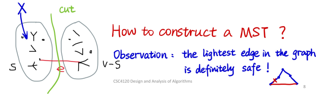
Prim最小生成树的实现细节和 Dijkstra 非常像,都是维护一个小根堆,每次贪心地加边。
Huffman 编码
用于无损压缩储存字符串,让一个字符串里面出现频率高的字符编码短,频率低的字符编码长一些,传统方法是所有字符编码长度一样。
Huffman树:一棵 $01$ 前缀二叉树,左 $0$ 右 $1$。
给定一组符号 $c_1, c_2, \cdots, c_n$ 和每个符号出现的频率(权值)$w_i$,目标是构建一棵二叉树,每个符号对应一个叶子节点,使得带权路径长度($W$)最小
$$ \text{minimize } W = \sum_{i=1}^n w_i \cdot \text{depth}(c_i) $$
核心思想(贪心):每次合并当前权值最小的两个节点。
还是用小根堆来维护。
而且 Huffman 编码通过构建前缀二叉树,保证了没有任何一个字符的编码是另一个字符编码的前缀,这样在解码的时候也不会有歧义。
解码就很简单了,直接对应 Huffman 树从根往下走,走到叶子节点就将其输出,然后再回到根。
动态规划
之前写过两篇 blog 关于 DP 的,可以简单参考一下
动态规划就是把一个复杂的大问题,拆解成一个个重复的小问题,并把小问题的答案记录下来,最后得到大问题的答案。
最重要的是无后效性,即“未来与过去无关,只与现在有关”。一旦某个状态被确定,它是怎么到达这个状态的,无关紧要!后续的决策只依赖于当前状态。
如何设计一个 DP 方程:
- 定义状态(State):为了描述当前的局面,我需要知道哪些变量?状态必须包含所有“会限制未来决策”的信息。
- 定义选择(Choice):在当前状态下,我能进行什么操作?
- 明确 DP 数组的含义(Definition):用语言将 $dp[\dots]$ 的定义写下来,一定要具体。
- 写出状态转移方程(Transition):把选择变成数学公式,通常是
min,max或者sum。
$$ 现在的状态=择优 (之前的状态+本次选择的代价/收益) $$
Floyd 算法(多源最短路)
定义 $$ dp^{(k)}[i][j]=只允许使用 {1,2,\cdots,k} 作为中间点时,i \to j 的最短路 $$
状态转移方程 $$ dp^{(k)}[i][j] = \min\{dp^{(k-1)}[i][j], dp^{(k-1)}[i][k] + dp^{(k-1)}[k][j] \} $$
int n, m;
int d[MAXN][MAXN];
bool findN;

void Floyd() {
	findN = false;
	for(int k = 1; k <= n; k++)
		for(int i = 1; i <= n; i++)
			for(int j = 1; j <= n; j++)
				if(d[i][k] < INF && d[k][j] < INF)
					d[i][y] = min(d[i][j], d[i][k] + d[k][j]);
	for(int x = 1; x <= n; x++)
		if(d[x][x] < 0) findN = true; // 找到负环
}
区间 DP
核心思想:大区间的解=小区间的解+合并代价
标准套路:定义 $dp[i][j]$ 表示区间 $[i, j]$ 经过一系列操作之后得到的最优解。
状态转移方程:为了求 $dp[i][j]$,我们把区间 $[i, j]$ 从中间切一刀,分成 $[i, k]$ 和 $[k+1, j]$,枚举这个分割点 $k$,找到最优解。
$$ dp[i][j] = \min_{i \leq k < j}{ dp[i][k] + dp[k+1][j] } + \text{Cost}(i, j) $$
其中,$\text{Cost}(i, j)$ 是将两部分合并产生的代价。
遍历顺序:按照区间长度从小到大枚举。先算长度 $1$ 的区间,再算长度 $2$ 的区间,以此类推,最后能得到整个大区间的最优解。
最长公共子序列 LCS
给定两个字符串,找到它们的最长公共子序列(不要求连续)。
状态转移方程: $$ dp[i][j] = \begin{cases} dp[i-1][j-1] + 1 & \text{if } s1[i] = s2[j] \\ \max \{dp[i-1][j], dp[i][j-1] \} & \text{otherwise}\end{cases} $$ 其中 $dp[i][j]$ 表示 $s1$ 的前 $i$ 个字符和 $s2$ 的前 $j$ 个字符的 LCS 长度。
旅行商问题 TSP
定义状态 $dp[mask][i]$: $mask$ 是一个二进制转化成十进制的数,其 $n$ 位二进制表示已经访问过的城市集合;$i$ 表示当前停留在哪个城市(一定要在 $mask$ 里)。其值表示从起点出发,访问了 $mask$ 里所有城市,最后停在 $i$ 的最小总距离。
状态转移:假设我们在状态 $dp[mask][i]$,那么上一步我们在一个没访问 $i$ 之前的状态,停在某个 $j$。
之前的集合 $prev\_ mask$ 可以表示为 $mask \text{ xor } (1 << i)$,也就是把 $mask$ 里第 $i$ 位的 $1$ 去掉。
那么状态转移方程: $$ dp[mask][i] = \min_{j \in prev\_ mask} \{dp[prev\_ mask][j] + d[j][i] \} $$
void TSP() {
    cin >> n;
    for (int i = 0; i < n; i++)
        for (int j = 0; j < n; j++)
            cin >> w[i][j];
    int full = (1 << n);
    for (int mask = 0; mask < full; mask++)
        for (int i = 0; i < n; i++)
            dp[mask][i] = INF;
    dp[1 << 0][0] = 0;

    for (int mask = 0; mask < full; mask++) {
        if (!(mask & 1)) continue;
        for (int i = 0; i < n; i++) {
            if (!(mask & (1 << i))) continue;
            int prev = mask ^ (1 << i);
            if (prev == 0 && i != 0) continue;
            for (int j = 0; j < n; j++) {
                if (!(prev & (1 << j))) continue;
                dp[mask][i] = min( dp[mask][i], dp[prev][j] + w[j][i]);
            }
        }
    }

    int ans = INF, all = full - 1;
    for (int i = 1; i < n; i++) {
        ans = min(ans, dp[all][i] + w[i][0]);
    }
    cout << ans << "\n";
}
背包问题
01 背包:
有 $n$ 个物品,物品重量 $w_i$,价值 $v_i$,每个物品最多只能拿一个,背包大小 $S$。 $$ dp[i][j] = \max\{dp[i-1][j], dp[i-1][j-w[i]]+v[i] \} $$ 其中 $dp[i][j]$ 表示前 $i$ 个物品在容量 $j$ 下的最大价值。
void Knapsack01() {
    int S, n;
    cin >> S >> n;
    for(int x = 1; x <= n; x++) cin >> w[x] >> v[x];
    for(int j = 0; j <= S; j++) {
        for(int i = 1; i <= n; i++) {
            if(j-w[i] < 0) dp[i][j] = dp[i-1][j];
            else dp[i][j] = max(dp[i-1][j], dp[i-1][j-w[i]] + v[i]);
        }
    }
    cout << dp[n][S] << endl;
}
时间复杂度 $O(nS)$
完全背包:
同上,但可以重复拿 $$ dp[j] = \max \{dp[j-1], \max_i{dp[j-w[i]]+v[i] } \} $$ 其中 $dp[j]$ 表示容量 $j$ 下的最大价值。
void KnapsackComplete() {
    int S, n;
    cin >> S >> n;
    for(int x = 1; x <= n; x++) cin >> w[x] >> v[x];
    for(int j = 0; j <= S; j++) {
        for(int i = 1; i <= n; i++) {
            if(j-w[i] >= 0)
                dp[j] = max(dp[j], dp[j-w[i]] + v[i]);
        }
    }
    cout << dp[S] << endl;
}
时间复杂度 $O(nS)$
平衡划分问题
给定一个包含 $n$ 个正整数的集合,如何将其划分为两个子集,使得这两个子集的元素和相差最小。
$$ \min_{S_1, S_2} d = \left| \sum_{i \in S_1} k_i - \sum_{j \in S_2} k_j \right| $$
核心解法:将其转化为 01 背包问题。先算出总和 $\text{Sum}$,找到一个子集使其和尽可能接近 $\frac{\text{Sum}}{2}$,然后就是一个容量为 $\frac{\text{Sum}}{2}$ 的 01 背包问题了,每个物品的价值和重量都是它本身,EZ。
网络流
想象一个由管道组成的网络:
- 源点(Source, $S$):自来水厂,有无限的水流出
- 汇点(Sink, $T$):大海,可以接收无限的水
- 容量(Capacity, $c$):每根管道 $(u,v)$ 单位时间最多能流过的水量
- 流量(Flow, $f$):实际流过的水量
还有以下规则:
- 流量限制:$f(u,v) \leq c(u,v)$(水管不能撑爆)
- 流量守恒:对于除了 $S$ 和 $T$ 以外的任意节点,流入量=流出量
那么问题:在不撑爆任何管道的前提下,从源点 $S$ 最多能推多少水到汇点 $T$?
Ford-Fulkerson 方法
核心思想:只要还能找到一条路去推流,就往死里推;推不动了,现在的流量就是最大流。
这条“能推流的路”叫做增广路(Augmenting Path)
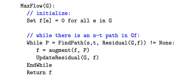
反向边:如果随便找了一条路推流,可能会堵死另一条更优的路线,那么可以加一个反向边,每当我们在边 $(u,v)$ 上推了 $k$ 的流量:
- 正向边的 $c(u,v)$ 减少 $k$
- 反向边的 $c(v,u)$ 增加 $k$
在残量网络(Residual Graph)中走反向边,相当于“撤销”之前的操作!
Edmonds-Karp 算法
用 BFS 在参量网络图里寻找增广路,确保每次找的都是边数最少的路。
这里的增广路是包括反向边的,但要满足硬性条件:剩余容量(Capacity)$>0$
BFS 总能找到经过边数最少的那条增广路(最短路性质),可以保证效率是 $O(nm)$,然后再乘上更新一次推流的复杂度 $O(m)$,使得算法总复杂度 $O(nm^2)$
LL BFS()
{
	memset(last, -1, sizeof(last));
	queue <LL> q;
	q.push(s);
	flow[s] = INF;
	while(!q.empty())
	{
		int u = q.front(); q.pop();
		if(u == t) break;
		for(LL x = head[u]; x > 0; x = edge[x].next)
		{
			LL v = edge[x].to, w = edge[x].w;
			if(w > 0 && last[v] == -1)
			{
				last[v] = x;
				flow[v] = min(flow[u], w);
				q.push(v);
			}
		}
	}
	return last[t] != -1;
}

LL EK()
{
	LL ans = 0;
	while(BFS())
	{
		ans += flow[t];
		for(LL x = t; x != s; x = edge[last[x] ^ 1].to)
		{
			edge[last[x]].w -= flow[t];
			edge[last[x]^1].w += flow[t];
		}
	}
	return ans;
}
代码是古早时期用链式前向星随便写的,凑合着看吧(
最大流最小割定理
Max-Flow Min-Cut Theorem
割的定义是顶点的集合,在网络流中特指 $s-t$ 割,即我们将顶点集合 $V$ 划分成 $S$ 和 $TY$,使得:
- 源点 $s \in S$
- 汇点 $t \in T$
- $S \cup T = V$ 且 $S \cap T \empty$
割的容量,记为 $C(S,T)$,是指所有从 $S$ 指向 $T$ 的边的容量之和。 $$ C(S,T) = \sum_{u \in S, v \in T} c(u,v) $$
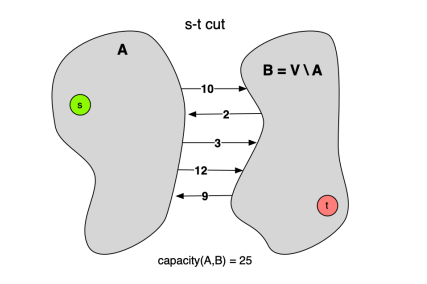
复杂度
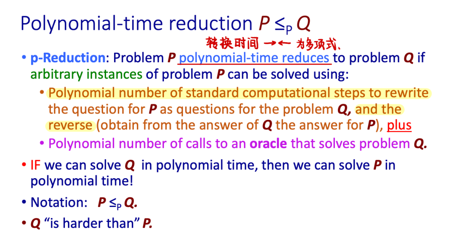
以下内容由 Gemini 生成
这四个概念(P, NP, NP-Hard, NP-Complete)是理论计算机科学的基石,但名字起得非常容易让人误解。
最常见的误区是:“NP 就是 Not Polynomial(非多项式),就是难解的问题。” —— 这是大错特错的!
我们要用验算和归约这两个视角来彻底搞懂它们。
1. P (Polynomial Time) —— “能做出来的”
定义:能在多项式时间 $O(n^k)$ 内解决的问题。 直观:计算机能快速搞定的问题。
- 例子:
- 给你一个数组,把它排个序。(归并排序 $O(n \log n)$)
- 给你个地图,找两点间最短路。(Dijkstra $O(E \log V)$)
- 判断一个数是不是偶数。($O(1)$)
2. NP (Nondeterministic Polynomial Time) —— “能检查答案的”
名字误区:NP 不代表“非多项式(Non-Polynomial)”,它代表“非确定性多项式(Non-deterministic Polynomial)”。这个名字来源于非确定性图灵机,比较抽象,你可以直接忽略它。
真正的定义(验证视角): 如果在多项式时间内,给定一个“解(Certificate/Witness)”,你能验证这个解是不是对的,那这个问题就在 NP 里。
直观:虽然我不会做,但如果你蒙了一个答案给我,我能很快告诉你蒙得对不对。
- 例子(数独):
- 让你解一个 $100 \times 100$ 的空数独,这极难(可能是指数级时间)。
- 但是,如果我直接塞给你一张填满了数字的纸,问你“这是不是解?”,你只需要扫描一遍行、列、宫,几秒钟就能告诉我 Yes 或 No。
- 所以,数独属于 NP。
P 和 NP 的关系:
- $P \subseteq NP$。
- 为什么?因为如果你能快速解出问题,那你当然也能快速验证答案(直接解一遍对比一下就行了)。
- 千古之谜:$P = NP$ 吗?(即:所有能被快速验证的问题,都能被快速解决吗?目前绝大多数科学家认为 $P \neq NP$)。
3. NP-Hard —— “大Boss”
定义:如果所有的 NP 问题都能在多项式时间内归约到问题 X,那么 X 就是 NP-Hard。
通俗翻译: “我是个狠角色。如果谁能把我也在多项式时间内解决了,那么世界上所有的 NP 问题(比如数独、TSP、图着色)就全都解决了。”
特点:
- 它不一定在 NP 里:NP-Hard 问题甚至可能连“验证答案”都很难。
- 它代表了“难度下限”:它至少和 NP 中最难的问题一样难。
- 例子:
- 停机问题:给定一段代码,判断它会不会死循环。这是不可解的,它比所有 NP 问题都难,所以它是 NP-Hard,但它不是 NP(因为连验算都做不到)。
4. NP-Complete (NPC) —— “NP 里的扛把子”
定义:一个问题如果满足两个条件,它就是 NPC:
- 它属于 NP(能被快速验证)。
- 它属于 NP-Hard(所有 NP 问题都能归约给它)。
直观: 它是 NP 集合里最难、最核心的那一小撮问题。它们处于 P/NP 图解的交界处。 NPC 问题的神奇之处在于它们的等价性:只要你解决了其中任何一个 NPC 问题(找到多项式算法),你就解决了所有的 NP 问题(即证明了 P=NP)。
- 经典 NPC 例子:
- SAT (布尔可满足性问题):第一个被证明是 NPC 的问题(祖师爷)。
- TSP (旅行商问题-判定版):给一个长度 $L$,问有没有一条路径长度小于 $L$?
- 最大团问题:图里有没有 $K$ 个点两两相连?
- 背包问题。
5. 总结与辨析(一张表看懂)
| 类别 | 核心能力 | 通俗理解 | 典型例子 |
|---|---|---|---|
| P | 能解决 | 简单题,电脑跑得飞快 | 排序、最短路、最小生成树 |
| NP | 能验证 | 只有上帝或欧皇能猜中答案,但我能检查对不对 | 数独、因数分解、以及所有 P 问题 |
| NPC | 能验证 + 最难 | NP 里的万恶之源。解出一个就能解出所有。 | SAT、TSP(判定)、图着色 |
| NP-Hard | 未必能验证 + 极难 | 难度无上限,包含了 NPC 和比 NPC 更难的问题 | 停机问题、TSP(优化版)、围棋必胜策略 |
6. 一个常考的细节:优化 vs 判定
通常我们在算法书上讨论 P/NP 时,讨论的都是判定问题(Decision Problem),即答案只有 Yes/No 的问题。
- TSP 优化版:“求最短路径是多少?” $\to$ 这是 NP-Hard。
- TSP 判定版:“是否存在一条路径长度 $< 100$?” $\to$ 这是 NP-Complete。
为什么? 因为“优化版”不好验证。如果我给你一条路,说“这是最短的”,你怎么验证它是最短的?你很难在多项式时间内验证没有更短的路。 但“判定版”很好验证。我给你一条小于 100 的路,你算一下长度,确实小于 100,验证通过。
总结
- P:做起来容易。
- NP:检查起来容易。
- NPC:NP 里最难的,如果攻克它,世界将发生巨变(密码学崩溃)。
- NP-Hard:只要能把所有 NP 问题转化成它,它就是 NP-Hard。
下次有人问你,你可以装作很深沉地说:“P 是解的集合,NP 是验证的集合,NPC 是这帮验证问题里的终极代理人。”
CSC3060 Introduction to Computer Systems
https://github.com/ghskyzhou/CSC3060-Note-Plus
感谢 DFT、MTC、LXY、ZXY 等同学的资源共享😭
当然也得感谢 Prof.Hsu 的 PPT
CSC3170 数据库系统 Database System
Part 1 简介 Introduction
结构化和非结构化的文本信息 Structured and Unstructured Textual Information
一个数据库管理系统(Database Management System, DBMS)是一个复杂的软件系统,其任务是帮助管理大量复杂的结构化信息。
结构化信息通常由离散的单元(实体 Entities)组成。
相同类型的实体会有预设的组织方案:
- 相同数量的性质 Attributes
- 每个性质都有预设的格式
非结构化的信息通常指没有固定格式、没有区分信息的数据,一般为普通的文本。
数据库系统 Database System
包含信息的数据集合叫做数据库。
其应用非常广泛,包括但不限于:
- 销售:顾客、产品、购买
- 会计:支付、发票
- 人力资源:应聘者信息、销售人员、税收
- 管理层
- 银行和金融
- 大学
数据库的目的是什么?主要是为了高效地存储、维护和查找大量数据,而且要保证不出现安全问题。
数据视图 View of Data
数据库系统是一些相互关联的数据以及一组使得用户可以访问和修改这些数据的程序的集合,其主要目的是给用户提供数据的抽象视图。
数据模型 Data Model
数据模型是描述数据、数据联系、数据语义以及一致性约束的概念工具的集合。其可以被划分为四类:
- 关系模型(Relational Model):利用表的集合来表示数据和数据间的联系,是最广泛的数据模型。
- 实体-联系模型(Entity-relationship Model):主要用作数据库设计。
- 半结构化数据模型(Semi-structured Data Model):允许数据定义中某些相同类型的数据项含有不同的属性集,例如 JSON, XML。
- 基于对象的数据模型(Objecte-based Data Model):面向对象的程序设计,例如 Java, C++, C#。
下面这个图是最常见的关系模型例子:
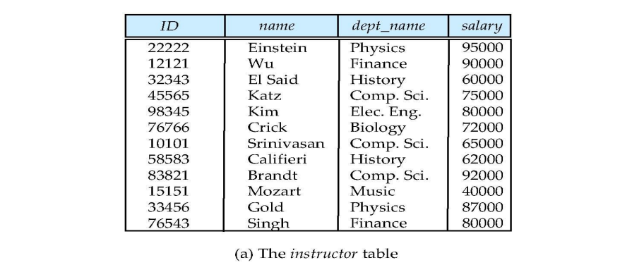
数据抽象 Data Abstraction
一个可用的系统必须要能高效地检索数据,系统开发人员通过如下几个层次的数据抽象来对用户屏蔽复杂性,以简化交互:
- 物理层(Physical Level):最低层次的抽象,描述数据实际上是怎样储存的。
- 逻辑层(Logical Level):描述数据库中存什么数据以及这些数据间存在什么联系。
- 视图层(View Level):只描述整个数据库的某个部分。
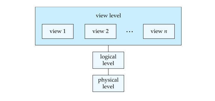
实例和模式 Instances and Schemas
随着时间的推移,信息会被插入或删除,数据库也就发生了改变。特定时刻存储在数据库中的信息的集合称作数据库的一个实例 Instance,而数据库的总体设计称作数据库模式 Schema。
数据库有几种模式:
- 物理模式(Physical Schema),在物理层描述数据库的设计。
- 逻辑模式(Logical Schema),在逻辑层描述数据库的设计。
- 子模式(Subschema),描述数据库的不同视图。
物理数据隔离 Physical Data Independence:在不改变逻辑模式的情况下改变物理模式的能力。
数据库语言 Database Language
数据定义语言 Data Definition Language (DDL)
定义数据库模式的专用标记,例如:
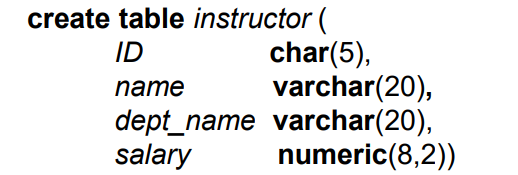
DDL 编译器会生成一系列表格模板,存在数字典 Data Dictionary 里。
数据字典包含元数据 Metadata:
- 数据库模式
- 完整性约束 Integrity Constraints
- Primary Key
- 授权
- 验证谁可以访问
数据操纵语言 Data Manipulation Language (DML)
可以使得用户访问或操纵,那些按照某种适当的数据模型组织起来的数据,通常也叫做查询语言。基本上有两种类型:
- 过程化的 DML(Procedural DML),要求用户指定需要什么数据以及如何获得这些数据
- 声明式的 DML(Declarative DML),只要求用户指定需要什么数据,不必指明如何获得
声明式的 DML 通常也被称为非过程化的 DML。
结构化的查询语言 Structured Query Language (SQL)
SQL 是非过程化的,一个查询包含输入一个或多个表格,返回一个表格。例子:
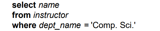
数据库设计 Database Design
设计数据库通常结构的流程:
- 逻辑设计 Logical Design:决定数据库模式。数据库设计要求我们能找到一个“好的”关系模式。
- 物理设计 Physical Design:决定数据库的物理层。
数据库组成 Database Components
一个数据库系统可以被划分成以下几个功能性模块:
- 储存管理器 Storage Manager
- 查询处理器 Query Processor
储存管理器 Storage Manager
储存管理器是数据库系统中负责在数据库中储存的低层数据与应用程序以及向系统提交的查询之间提供接口的部件。
储存管理器负责以下任务:
- 与操作系统文件管理器交互
- 高效地储存、检索和更新数据
储存管理器实现了以下几种数据结构:
- 数据文件(Data File):储存数据库它本身
- 数据字典(Data Dictionary):储存数据库结构的元数据
- 索引(Index):能提供对数据项的快速访问
查询处理器 Query Processor
查询处理器组件包括:
- DDL 解释器(DDL Interpreter):解释 DDL 语句并将这些定义记录在数据字典中
- DML 编译器(DML Compiler):将查询语言中的 DML 语句翻译为包括一系列查询执行引擎能理解的低级指令的执行方案
- 一个查询通常可以被翻译成给出相同结果的多个候选执行计划中的任何一个。DML 编译器还进行查询优化(Query Optimization),就是从几个候选执行计划中选择代价最小的那个执行计划。
- 查询执行引擎(Query Evaluation Engine):它执行由 DML 编译器产生的低级指令。
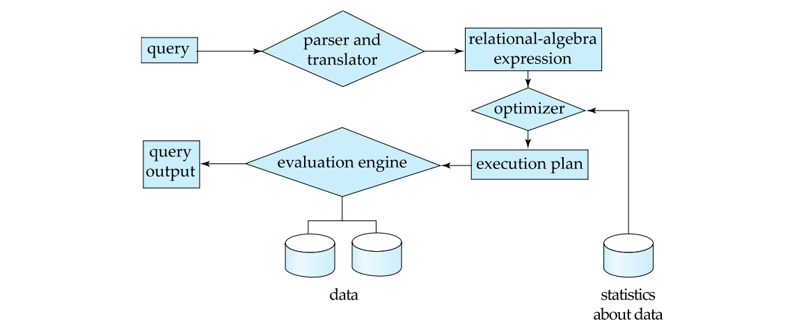
事务管理 Transaction Management
事务 Transaction是数据库应用中完成单一逻辑功能的操作集合。
数据库架构 Database Architecture
- 中心化的数据库
- 一些核心,共享内存
- 客户端-服务器
- 一个服务器机器执行基于多个客户端的工作
- 平行数据库
- 多核,共享内存
- 共享硬盘
- 什么都不共享
- 分布式数据库
- 地理上的分布
- 模式 / 数据异质性
数据库用户和管理员 Database Users and Administrator
数据库用户:
- 普通(初学者=)用户
- 应用程序员
- 复杂(老练)用户
数据库管理员:
- 模式定义
- 存储结构及存取方法定义
- 模式及物理组织的修改
- 数据访问授权
- 日常维护
Part 2 关系模型介绍 Introduction to Relational Model
关系数据库由表 Table的集合构成,每张表被赋予一个唯一的名称。
一个关系表的例子:
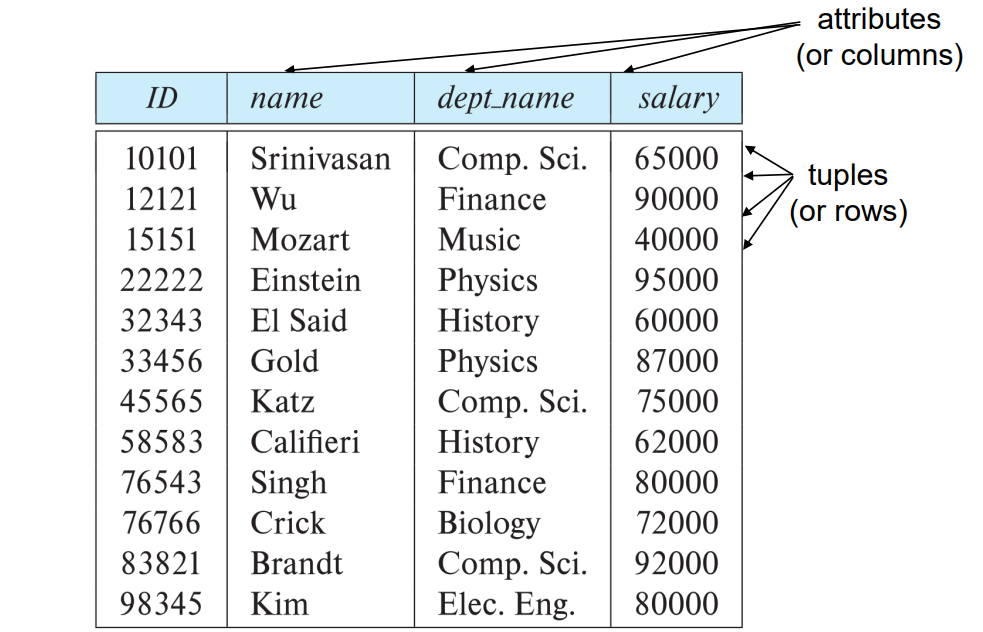
关系的数学定义 Mathematical Definition of Relation
笛卡尔积 Cartesian Product
考虑两个任意集合 $A$ 和 $B$,包括所有有序对 $(a,b), a \in A, b \in B$ 的集合叫做 $A$ 和 $B$ 的笛卡尔积。 $$ A \times B = {(a,b):a \in A, b \in B} $$ 如果 $A=B$,我们通常将 $A \times A$ 写成 $A^2$。
- e.g. 如果$A = \mathbb{R}$,那么 $\mathbb{R}^2$ 就是二维笛卡尔平面。
记集合 $A$ 的基数 Cartesian 为 $|A|$,则有 $$ |A \times B| = |A| \times |B| $$
从 $A$ 到 $B$ 的一个二元关系 Binary Relation $R$,就是 $A \times B$ 的一个子集,即 $R \subseteq A \times B$
一般来说,定义在集合 $D_1,D_2,\cdots,D_n$ 上的 $n$ 元关系 n-ary Relaion $R$ 是笛卡尔积 $$ D_1 \times D_2 \times \cdots D_n $$ 的一个子集,即 $$ R \subseteq \prod_{k=1}^n D_k $$ 其中,$D_1,D_2,\cdots,D_n$ 通常被称为域 Domain。
并且该笛卡尔积的基数为 $$ \left| \prod_{k=1}^n D_k \right| = \prod_{k=1}^n \left| D_k \right| $$ 也就是说,笛卡尔积的元素个数等于各个集合基数的乘积。
如果某个特定元组 tuple 出现在关系 $R$ 中,就表示该元组所表达的信息在当前是真实且有效的信息。
举个例子,假设
- $D_1=$ 学号
- $D_2=$ 学院
- $D_3=$ 生源城市 如果 $$ (114514, \text{CS}, \text{Shenzhen}) \in R $$ 表示学号为 $114514$ 的学生属于 CS 学院,并且来自深圳。但是 $$ (114515, \text{CE}, \text{Guangzhou}) \notin R $$ 表示“学号为 $114515$ 的学生属于 CE 且来自广州”这一说法不成立。
关系模式和实例 Relation Schema and Instance
$A_1, A_2, \cdots, A_n$ 被称为属性 attributes。
$R(A_1, A_2, \cdots, A_n)$ 被称为关系模式 relation schema,有时也被称为关系方案 relation scheme,它由关系名和属性列表组成,这些属性对应表中的列 columns。
- e.g. instructor(ID, name, dept_name, salary)
定义在关系模式 $R$ 上的关系实例 relation instance(也被称为关系状态 relation state)记为 $$ r(R) $$ 它由实际的数据值组成
- 一个关系当前的取值通常通过一张表 table 来表示
关系 $r$ 中的一个元素 $t$ 被称为元组 tuple,在表中用一行 row 来表示。
模式描述的是逻辑结构,而实例时某一时刻数据的快照。
例如下图
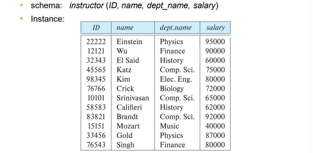
属性 Attributes
每个属性允许取值的集合称为该属性的域 domain。
属性值通常要求是原子性的 atomic,即不可再分的。
特殊值 null 被认为时每个域中搞的一个成员,表示该值未知。
null 值会使许多数据库操作的定义变得更加复杂。
键 Keys
设 $K \subseteq R$,如果属性集合 $K$ 的取值足以认证唯一标识关系 $R$ 的一个元组 tuple,则称 $K$ 为 $R$ 的一个超键 superkey。
- e.g. ${\text{ID}}$ 和 ${\text{ID}, \text{name}}$ 都是关系 instructor 的超键。
如果一个超键 $K$ 是最小的 minimal,则称之为候选键 candidate key。
- e.g. ${\text{ID}}$ 是 instructor 的一个候选键。
在所有候选键中,会选择一个作为主键 primary key。
外键 foreign key 约束:一个关系中的某个值必须出现在另一个关系中。
- 引用关系 referencing relation
- 被引用关系 referenced relation
关系代数 Relational Algebra
关系代数由一组运算组成,这些运算接受一个或两个关系作为输入,并生成一个新的关系作为它们的结果。
六个基础运算符:
- 选择 select:$\sigma$
- 投影 project:$\Pi$
- 集合并 union / 交 intersection:$\cup$
- 集合差 set difference:$-$
- 笛卡尔积 Cartesian product:$\times$
- 更名 rename:$\rho$
选择运算 Select Operation
选择运算选出给定满足给定谓语的元组。
记号:$\sigma_p(r)$
其中,$p$ 被称作选择谓词 selection predicate。
- e.g. 选择满足在 Physics 部门的 instructor:
$$ \sigma_{\text{dept name="Physics"}}(\text{instructor}) $$
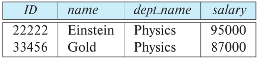
在选择运算中我们允许使用 $=,\not=,>,\geq,<,\leq$,也可以利用连接符号 $\land,\lor,\lnot$ 结合谓语。
- e.g. 选择满足在 Physics 部门且薪水高于 $90,000 的 instructor:
$$ \sigma_{\text{dept name="Physics" } \land \text{ salary > 90,000}}(\text{instructor}) $$
投影运算 Project Operation
投影运算是一种一元运算,返回它的参数关系,但滤掉了特定的属性。
记号:$\Pi_{A_1, A_2, A_3, \cdots, A_k} (r)$
其中 $A_1, A_2, A_3, \cdots, A_k$ 是属性名,$r$ 是关系名。
- e.g. 查询以下属性的 instructor
$$ \Pi_{\text{ID, name, salary}}(\text{instructor}) $$
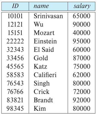
其实就是去掉了 dept_name。
关系运算的组合 Composition of Relational Operations
因为一个关系代数运算的结果也是关系,所以可以直接连接起来(就像函数括号),例如:
$$ \Pi_{\text{name}}(\sigma_{\text{dept name="Physics"}}(\text{instructor})) $$
笛卡尔积运算 Cartesian Product Operation
笛卡尔积运算用叉号 $\times$ 表示,允许我们结合来自任意两个关系的信息。其作用就是,假设现在有 $n$ 行的关系 $A$ 和 $m$ 行的关系 $B$,那么 $A \times B$ 就会得到一个 $n*m$ 的关系,$A$ 中的每一个关系都对应 $B$ 中的所有关系。
- e.g. instructor $\times$ teaches
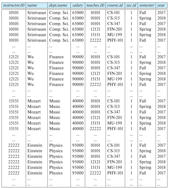
这里找不到原来两张表的电子版了,但大概就是能看出来是原来的一条左边的关系对应右边的所有关系,这样形成一个 $n*m$ 行的关系
连接运算 Join Operation
连接运算是我们能够选择与笛卡尔积合并到单个运算中。
考虑关系 $r(R)$ 和 $r(S)$,并令 $\theta$ 为 $R \cup S$ 模式的属性上的一个谓词。连接运算的定义是: $$ r \bowtie s = \sigma_\theta (r \times s) $$
- e.g. $\text{instructor} \bowtie_{\text{instructor.id = teaches.id}} \text{teaches} \\ = \sigma_{\text{instructor.id = teaches.id}}(\text{instructor} \times \text{teaches})$
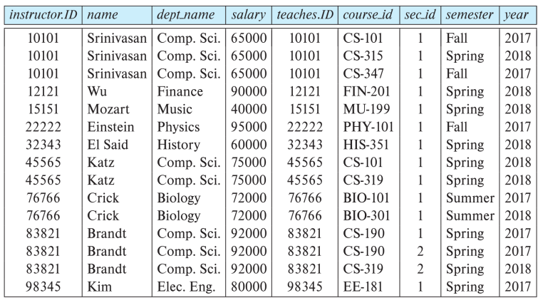
其实就是先做了笛卡尔积运算,再做一次选择运算。
集合运算 Set Operation
并运算 Union Operation
并运算使我们能够合并两个关系。
为了使并集运算有意义,必须要保证:
- 输入并运算的两个关系具有相同数量的属性,一个关系的属性数量被称为它的元数 Arity。
- 当属性有关联的类型时,对于每个 $i$,两个输入关系的第 $i$ 个属性的类型必须相同。
这样的关系被称为相容 Compatible 关系。
记号:$r \cup s$
交运算 Intersection Operation
交运算允许我们找到同时出现在两个输入关系中的元组。
与并集运算一样,我们要保证交是在相容关系之间进行运算的。
记号:$r \cap s$
集差运算 Set-Difference Operation
集差运算能使我们找到在一个关系中但不在另一个关系中的元组。
与并集运算一样,我们要保证集差是在相容关系之间进行运算的。
记号:$r - s$
因为教授的 PPT 上并没有很好的例子图示,在这里就不给出了,而且这三个集合运算也很好理解。
赋值运算 Assignment Operation
有时候通过将一个关系代数表达式中的一部分赋值给临时的关系变量,可以方便地编写该表达式,赋值运算用 $\leftarrow$ 表示,其工作方式类似于程序语言中的赋值。
- e.g. 找到所有在 Physics 和 Music 部门的 instructor $$ \begin{align*} &\text{Physics} \leftarrow \sigma_{dept name="Physics"}(instructor) \\ &\text{Music} \leftarrow \sigma_{dept name="Music"}(instructor) \ &\text{Physics} \cup \text{Music} \end{align*} $$
更名运算 Rename Operation
关系表达式的结果并没有可以用来指代它们的名称,更名运算使我们能够做到这一点。
记号:$\rho_x(E)$
能返回以 $x$ 命名的表达式 $E$ 的结果。
Part 3 实体-联系模型 The Entity-Relationship Model
实体-联系数据模型(E-R 数据模型)被开发来方便数据库的设计,它是通过允许定义代表数据库全局逻辑结构的企业模式 Enterprise Schema 来做到的。
E-R 数据模型包含下面三个基本概念:
- 实体集 Entity Sets
- 关系集 Relationship Sets
- 属性 Attributes
实体集 Entity Sets
实体 Entity 是现实世界中可以区分于所有其它对象的一个“事物”或“对象”。
- e.g. 特定的人,公司,活动
实体集 Entity Set 是共享相同性质或属性的、具有相同类型的实体的集合。
- e.g. 所有人的集合,公司集合,产品
实体通过一组属性 Attributes 来表示,属性是实体集中每个成员所拥有的描述性性质。
- e.g. $\text{instructor}=(\text{ID, name, salary})$
属性的子集构成了一个实体集的主键 Primary Key,即它可以唯一认定集合的元素。
实体集在 ER 图里的表示:
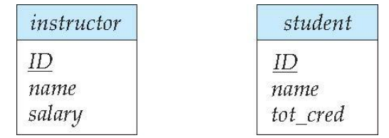
关系集 Relationship Sets
联系 Relationship 是多个实体间的相互关联,关系集 Relationship Set 是相同类型联系的集合。
关系集的数学定义: $$ {(e_1, e_2, \cdots, e_n):e_1 \in E_1, e_2 \in E2, \cdots, e_n \in E_n } $$ 其中,$(e_1, e_2, \cdots, e_n)$ 是个联系。
例如,我们定义一个关系集 advisor 表示 student 和 instructor 之间的关联,然后我们就可以在实体之间连线。
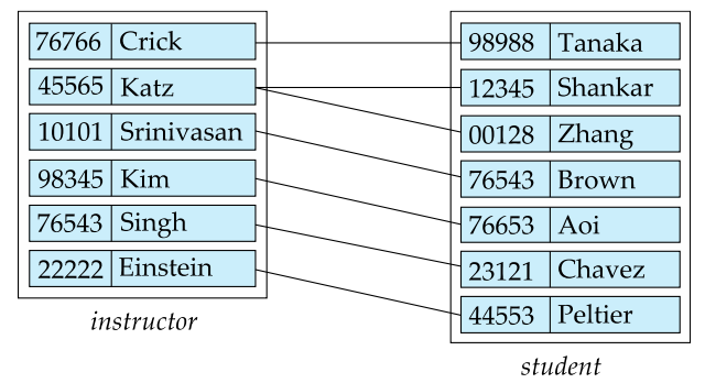
关系集在 ER 图里的表示:
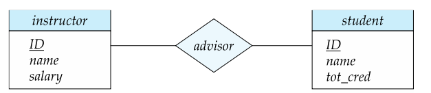
联系也可以具有被称作描述性属性 Descriptive Attribute 的属性。
例如下图,每个联系具有一个 date,表示 student 和 instructor 建立 advisor 联系的时间。
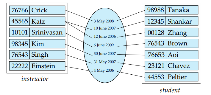
带有属性的关系集在 ER 图里的表示:
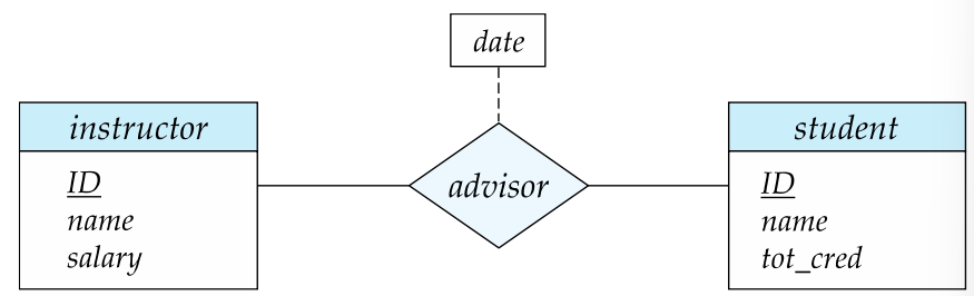
实体集的关系不需要是独特的,实体在联系中扮演的功能被称为实体的角色 Role。
下图中,course_id 和 prereq_id 被称作角色。
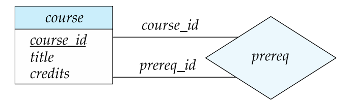
复杂属性 Complex Attributes
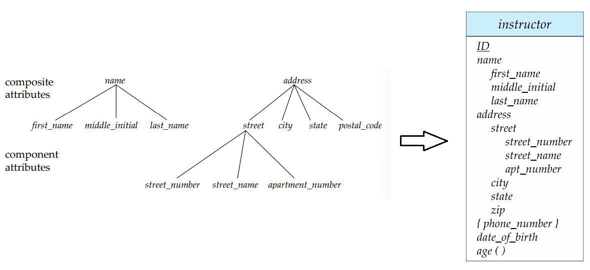
映射基数 Mapping Cardinality
映射基数 Mapping Cardinality 或基数比率表示一个实体能通过一个关系集关联的另一些实体的数量,多用于描述而二元关系集。
对于一个二元关系集来说,映射基数必然是以下情况之一:
- 一对一 One-to-one
- 一对多 One-to-Many
- 多对一 Many-to-one
- 多对多 Many-to-many
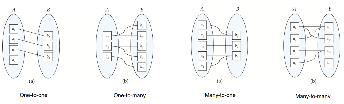
在 ER 图中,我们用单箭头直线($\rightarrow$)来表示“一”,用无箭头之间($-$)来表示“多”。下图从左上到右下分别是一对一、一对多、多对一、多对多。
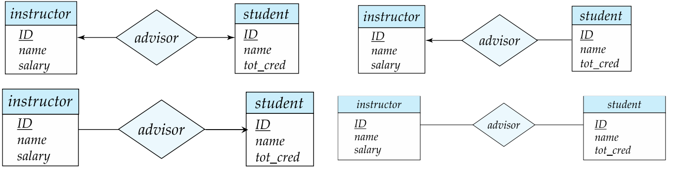
其中,一对一在这里的意思就是,一位导师最多可以指导一名学生,一名学生最多只能有一位导师;一对多在这里的意思就是,一位导师可以知道多名学生,但一名学生最多只能有一位导师;其余同理。
全部和部分参与 Total and Partial Participation
如果实体集 $E$ 中的每个实体都必须参与到关系集 $R$ 的至少一个联系中,那么实体集 $E$ 在关系集 $R$ 中的参与就被称为是全部的 Total,否则就被称为是部分的 Partial。
全部参与用双直线表示。
例如下图:
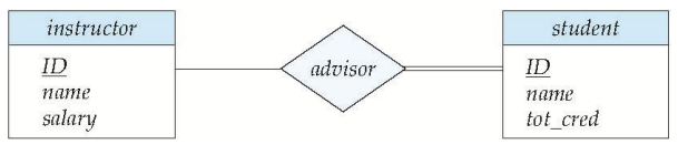
student 在 advisor 关系集中的参与是全部的,即每个学生都至少有一位导师。instructor 在 advisor 关系集中的参与是部分的,即一位导师不是必须要指导学生。
更复杂的约束 More Complex Constraints
线段上可以有一个关联的最小和最大基数,用 $l..h$ 的形式表示,其中 * 表没有限制。示例如下图:
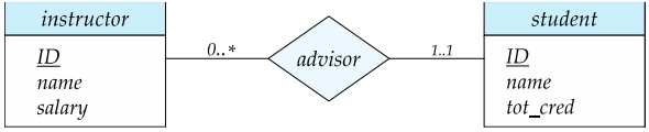
导师可以指导 $0$ 个或多个学生;一个学生至少有一个导师,无上限。
Generated by ChatGPT
下面从 Primary Key 开始,按你给出的课程结构一直讲到 Multivalued Dependency 与 Fourth Normal Form。我尽量保持 定义式、考试导向、少换行、逻辑紧凑的形式。
Part 3(后半)Primary Key, Weak Entity, Schema Representation
Primary Key(主键)
定义:在关系模式 (R) 中,若属性集合 (K) 满足以下两个条件,则称 (K) 为 Primary Key: (1) 唯一性(uniqueness):任意两个不同元组在属性 (K) 上的取值不同。 (2) 最小性(minimality):(K) 的任何真子集都不满足唯一性。
换句话说,Primary Key 是从 Candidate Keys(候选键) 中选出的一个作为主要标识符的键。Candidate Key 是所有满足唯一性与最小性的属性集合,而 Superkey 是任何能唯一标识元组的属性集合(不要求最小性)。因此关系为: Superkey ⊇ Candidate Key ⊇ Primary Key。
Prime Attribute 指属于某个 Candidate Key 的属性,Non-prime Attribute 指不属于任何 Candidate Key 的属性。
在关系模型中通常还涉及 Foreign Key:若关系 (R) 中属性集合 (F) 的值必须出现在另一关系 (S) 的 Primary Key 中,则称 (F) 为引用 (S) 的 Foreign Key。
Weak Entity Sets(弱实体集)
弱实体是 没有完整主键的实体集,其存在依赖于另一个实体集(称为 identifying entity)。弱实体的标识需要两个部分: (1) Partial Key(部分键):弱实体内部可区分对象的属性集合。 (2) Owner Entity 的 Primary Key。
因此弱实体的主键为: Owner Primary Key ∪ Partial Key。
例如:Employee(emp_id) 与 Dependent(name, age)。Dependent 无法仅通过 name 唯一标识,需要 (emp_id, name) 才能唯一确定一个 dependent。
在 ER 图中弱实体通常用 双矩形表示,identifying relationship 用 双菱形表示,且弱实体必须 total participation 于 identifying relationship。
Representing Schema(ER 到关系模式)
将 ER 模型转换为关系模式通常遵循以下规则: (1) 实体集 → 关系模式:实体的属性成为关系的属性,实体的主键成为关系的 Primary Key。 (2) 弱实体 → 关系模式:加入 owner entity 的主键作为外键并与 partial key 组成复合主键。 (3) 1:N relationship:在 N 端关系中加入 1 端的主键作为 Foreign Key。 (4) M:N relationship:建立新的关系模式,其属性为两个实体主键的并集(再加上关系属性)。 (5) relationship attributes:作为新关系模式中的属性出现。
Part 4 Extended Entity-Relationship Features
EER(Extended ER)模型在普通 ER 的基础上增加了 更复杂的建模能力,核心包括 specialization、generalization 与 aggregation。
Specialization(特化) 指从一个高层实体集派生出多个子实体集,每个子实体集具有额外属性或语义。例如 Person → Student、Employee。子类自动继承父类属性。
Generalization(泛化) 是 specialization 的逆过程,将多个实体抽象为一个更一般的实体。例如 Car 与 Truck 可以泛化为 Vehicle。
在 EER 中还涉及两个重要约束: (1) Disjointness constraint:子类之间是否互斥。若 disjoint,则一个实体最多属于一个子类;若 overlapping,则可属于多个子类。 (2) Completeness constraint:是否 total specialization。若 total,则每个父类实体必须属于某个子类;若 partial,则可以不属于任何子类。
另一个扩展概念是 Aggregation,用于表示“关系之间的关系”。例如 Manager 管理 Works_on 关系(员工参与项目),此时需要把 Works_on 看作一个高层对象参与新的关系。
Part 5 Relational Database Design and Normalization
关系数据库设计的目标是 减少冗余并避免更新异常(update anomaly)。常见异常包括: Insertion anomaly:无法插入某些信息而不引入无关数据; Deletion anomaly:删除数据时丢失其他有用信息; Update anomaly:同一事实需在多处修改。
为解决这些问题,需要进行 Normalization(规范化),即通过分析 Functional Dependencies(函数依赖) 将关系分解为多个结构更合理的关系模式。规范化通常涉及一系列范式(Normal Forms),如 1NF、2NF、3NF、BCNF、4NF 等。数据库设计通常希望达到 BCNF 或至少 3NF,同时保持 lossless join 与 dependency preservation。
Lossless Join 指将关系分解为多个关系后,通过自然连接可以恢复原关系。 Dependency Preservation 指原有函数依赖可以在分解后的关系中被直接验证。
Part 6 Functional Dependency Theory
Functional Dependency(FD) 是规范化理论的核心。
定义:在关系模式 (R) 中,属性集合 (X) 到属性集合 (Y) 的函数依赖记为 (X → Y),若对任意两个元组 (t_1,t_2),只要 (t_1[X] = t_2[X]),则必有 (t_1[Y] = t_2[Y])。
Trivial FD:若 (Y ⊆ X),则 (X → Y) 为平凡函数依赖。
Attribute Closure:给定属性集 (X) 和函数依赖集合 (F),闭包 (X^+) 是在 (F) 下由 (X) 可推出的所有属性集合。计算闭包的算法为:初始化 (X^+=X),若存在 FD (A→B) 且 (A ⊆ X^+),则加入 (B) 到 (X^+),重复直到不再变化。
闭包用于: (1) 判断 Candidate Key(若 (X^+) 包含所有属性,则 (X) 为 superkey); (2) 判断 FD 是否由 (F) 推导。
Armstrong’s Axioms 提供了推导函数依赖的基本规则: Reflexivity:若 (Y ⊆ X),则 (X → Y)。 Augmentation:若 (X → Y),则 (XZ → YZ)。 Transitivity:若 (X → Y) 且 (Y → Z),则 (X → Z)。
从这三条可推导出 union、decomposition、pseudo-transitivity 等规则。
3NF 与 BCNF
BCNF(Boyce–Codd Normal Form)定义:若对所有非平凡 FD (X → Y),都有 (X) 为 superkey,则关系模式在 BCNF 中。
Third Normal Form(3NF)定义:若对每个 FD (X → Y),满足以下之一: (1) (X) 是 superkey; (2) (Y) 为 prime attribute; (3) 该 FD 为 trivial。
BCNF 比 3NF 更严格。BCNF 能消除更多冗余,但分解后可能不保持依赖,而 3NF 保证存在 dependency-preserving decomposition。
Part 7 Multivalued Dependency and Fourth Normal Form
Multivalued Dependency(MVD) 表示为 (X →→ Y)。其含义是:若两个元组在 (X) 上相同,则可以交换它们在 (Y) 上的值而仍属于该关系。直观上表示:对于同一 (X),(Y) 的取值集合与其他属性是独立的。
例如关系 Student(student, skill, language),若学生的技能与语言互不影响,则存在 student →→ skill student →→ language。
这种情况下数据会出现冗余组合,例如若某学生有两种 skill 和两种 language,则需要存储四条记录。
Fourth Normal Form(4NF)定义:若对于每个非平凡 MVD (X →→ Y),都有 (X) 为 superkey,则关系模式在 4NF 中。
当存在违反 4NF 的 MVD 时,需要将关系分解。例如将 Student(student, skill, language) 分解为 StudentSkill(student, skill) 与 StudentLanguage(student, language)。
这种分解既消除了冗余,又保持无损连接。
Generated by Gemini Pro
Final Exam:
- 判断题、单选题、填空题、大题
- multivalue/function depengden
- 4nf/bcnf
- lossless decompose
- indexing
- b tree
- cap theorem(no sql)
- H base
- recovery track(undo...)
Part 7 Multivalued Dependency and Fourth Normal Form
收到,这份 Part 7 讲的是多值依赖 (MVD) 和 第四范式 (4NF)。
这份 PPT 看起来全都是希腊字母 $\alpha, \beta, \gamma$,但其实核心就是在解决一个开发中极容易碰到的傻逼设计:把两个完全不相干的 一对多 (1-to-N) 关系,硬塞到了同一张表里 。
核心拿分点(必考大题:4NF 分解与证明)
如果你在卷子上看到形如 $A \rightarrow \rightarrow B$ 的符号(中间是两个箭头),这就是在考 MVD 和 4NF。大题一定会让你把一张烂表无损分解 (Lossless Decomposition) 成 4NF 。
1. 什么是 MVD ($\alpha \rightarrow \rightarrow \beta$)?
-
大白话: 属性 $\alpha$ 决定了一组 $\beta$ 的值,并且这组 $\beta$ 的值跟表里的其他属性完全没有关系 。
-
PPT 例子: 一个老师 (ID) 有多个小孩 (child_name),也有多个电话 (phone_number) 。小孩和电话互不干涉。如果全塞进一张表
inst_info(ID, child_name, phone_number),就会出现恐怖的笛卡尔积(数据冗余) 。为了保持数据合法,你必须把小孩和电话的所有组合都列出来 。
2. 什么是 4NF?
- 判断标准: 对于表里的每一个非平凡的 MVD ($\alpha \rightarrow \rightarrow \beta$),左边的 $\alpha$ 必须是超码 (Superkey)(也就是说 $\alpha$ 能唯一确定一行记录)。如果 $\alpha$ 不是超码,这张表就不满足 4NF 。
3. 💥 必背拆表公式(4NF Decomposition Algorithm): 当一张表 $R$ 违背了 4NF(存在 $\alpha \rightarrow \rightarrow \beta$,但 $\alpha$ 不是超码),直接套这个公式把它劈开 :
-
新表 1: 包含 MVD 的左右两边 $\rightarrow (\alpha, \beta)$
-
新表 2: 左边 $\alpha$ 保留,加上表里剩下的所有属性 $\rightarrow (R - \beta)$
-
实战推导(参考 PPT 第 17 页): 已知 $R=(A,B,C,G,H,I)$,依赖有 $A \rightarrow \rightarrow B$、$B \rightarrow \rightarrow HI$、$CG \rightarrow \rightarrow H$ 。
-
第一步: 拿 $A \rightarrow \rightarrow B$ 开刀(A 不是超码,违背 4NF)。拆成 $R_1 = (A, B)$ 和 $R_2 = (A, C, G, H, I)$ 。
-
第二步: 检查 $R_2$。里面有个 $CG \rightarrow \rightarrow H$(CG 不是 $R_2$ 的超码)。把 $R_2$ 拆成 $R_3 = (C, G, H)$ 和 $R_4 = (A, C, G, I)$ 。
-
第三步: 检查 $R_4$。利用传递性,既然 $A \rightarrow \rightarrow B$ 且 $B \rightarrow \rightarrow HI$,所以推导出 $A \rightarrow \rightarrow HI$,在这个 $R_4$ 表里就是 $A \rightarrow \rightarrow I$ 。把 $R_4$ 拆成 $R_5 = (A, I)$ 和 $R_6 = (A, C, G)$ 。
4. 如何证明是无损分解 (Lossless Decomposition)?
-
判定条件: 拆出来的两个表 $R_1$ 和 $R_2$,它们的交集,必须能多值决定 (multi-determines) 其中任何一张表 。
-
公式: $R_1 \cap R_2 \rightarrow \rightarrow R_1$ 或者 $R_1 \cap R_2 \rightarrow \rightarrow R_2$ 必须成立 。
概念防坑指南(专门对付选择题 / 判断题)
- 平凡多值依赖 (Trivial MVD): 什么时候 MVD 是“平凡的”(也就是废话)?满足以下两点之一即可:
-
右边本来就是左边的子集 ($\beta \subseteq \alpha$) 。
-
这张表里只有这两个属性 ($\alpha \cup \beta = R$) 。
- FD vs MVD: 所有的函数依赖 (FD) 都是多值依赖 (MVD) 的特例。即如果 $\alpha \rightarrow \beta$ 成立,那么 $\alpha \rightarrow \rightarrow \beta$ 一定成立 。FD 要求只能有 1 个值(等值生成),MVD 允许有一组值(元组生成)。
- 4NF 和 BCNF 的关系: 只要一张表是 4NF,它绝对是 BCNF(4NF 条件更苛刻)。
- 反范式化 (Denormalization): 为什么有时候我们要故意违反范式,把数据塞在一张表里?纯粹是为了查询性能 (faster lookup),避免耗时的 JOIN 操作 。
Part 8 - 9 SQL
Skip
Part 10 NoSQL and Big Data Storage Systems
核心拿分点 1:CAP 定理(必考选择 / 简答题)
这个你在做后端架构时肯定听过,分布式系统的“不可能三角” 。教授非常喜欢考这三个字母的含义以及为什么只能“三选二” 。
-
C (Consistency 一致性): 强一致性。你往节点 A 写入了数据,立刻去节点 B 读,读到的必须是最新写入的数据 。
-
A (Availability 可用性): 只要系统没死绝,用户的请求就必须有响应(哪怕给的是旧数据),不能报错或无响应 。
-
P (Partition Tolerance 分区容错性): 哪怕节点之间的网线被挖断了(网络裂脑,分成了几个孤岛),系统依然要能继续运行 。
-
考场防坑逻辑: 在现实世界的分布式系统中,P(网络故障)是必然会发生的 。一旦发生网络分区,你要么为了保证 C(一致性)而拒绝服务(此时失去 A),要么为了保证 A(可用性)而返回各节点的旧数据(此时失去 C)。所以现实中往往采用最终一致性 (Eventual Consistency) 来保 A 和 P 。
核心拿分点 2:HBase 数据模型(极其容易考填空 / 对比题)
教授上一份透题里明确提到了 H base,这绝对是重头戏。你要抛弃 MySQL 那种固定的二维表思维。HBase 底层就是一个巨大的、稀疏的、多维的、嵌套的 Map (字典) 。
-
五维坐标定位: 在 HBase 里,要找到一个具体的数据(Cell),必须通过以下 5 个维度的 Key 来定位,请死记硬背这个 5-tuple 公式:
(Table, RowKey, ColumnFamily, ColumnQualifier, Timestamp)。如果查询时不写 Timestamp,默认返回最新版本的数据 。 -
Column Family (列族) vs Column Qualifier (列限定符):
- 列族 (Column Family): 建表的时候就必须定死,物理存储上同一个列族的数据存在一起 。
- 列限定符 (Column Qualifier): 极其灵活,插入数据时动态生成(比如你突然想存个微信号,直接插就行,不需要 ALTER TABLE) 。
- 它们组合成具体的列:
Family:Qualifier(例如Name:Fname或Details:Job) 。
-
Row Key (行键): HBase 里的数据是严格按照 Row Key 的字典序 (lexicographically) 排列的 。
核心拿分点 3:MapReduce 执行流程(大题预警)
如果教授要考 Big Data 的计算题,90% 的概率是让你手写或推导 MapReduce 的 Word Count(词频统计)流程 。只要记住这三个核心阶段的输入输出长什么样就行。
假设输入文件有两行:Deer Bear River 和 Car Car River 。
- Map 阶段(各干各的): Worker 读取自己分到的数据,把每一个单词拆出来,不管三七二十一,直接输出一个带数字 1 的键值对 。
- 输出:
(Deer, 1),(Bear, 1),(River, 1),(Car, 1),(Car, 1),(River, 1)。
- 输出:
- Shuffle 阶段(系统自动完成的洗牌): 把所有 Map 输出的键值对,按照 Key (单词) 进行分组和合并,把相同 Key 的 Value 塞进一个列表里发给对应的 Reduce 机器 。
- 系统输出:
(Car, [1, 1]),(River, [1, 1]),(Deer, [1]),(Bear, [1])。
- 系统输出:
- Reduce 阶段(汇总收网): 针对每一个 Key,把它的 Value 列表里的数字全加起来 。
- 最终输出:
(Car, 2),(River, 2),(Deer, 1),(Bear, 1)。
- 最终输出:
核心概念(选择题扫一眼就行)
-
Sharding (分片): 把一个几亿条记录的表,按照某个规则(比如 UserID)切成好几块,分别存放在不同的服务器上,用来分摊读写压力(负载均衡) 。
-
MongoDB: 基于文档 (Document-based) 的 NoSQL,存的实际上是 JSON 对象 。Schema-less(无模式),同一个表里的每一行数据结构可以完全不一样 。
-
HDFS (Hadoop File System): 它是分布式文件系统。主节点叫 NameNode(只存目录和块的映射信息,不存真数据),从节点叫 DataNode(存真实的硬盘块) 。为了防灾,每个数据块默认存 3 份 。
Part 11 File Organization and Indexing
这份 Part 11 讲的是文件组织和索引 (File Organization and Indexing)。
这章没有复杂的数学计算,全是纯纯的底层存储概念。你平时配过 Ubuntu 服务器、搞过自建图床,其实对文件系统和磁盘 I/O 的瓶颈肯定有感觉。数据库最怕的就是频繁读写磁盘(I/O 极慢),所以这章所有的设计,目的只有一个:减少磁盘 I/O 次数。
这章主要出选择题、判断题,极少数会考简答。直接看下面的干货拆解:
核心拿分点(必考概念辨析)
教授最喜欢把下面这两对概念混在一起考你:
-
稠密索引 (Dense Index) vs 稀疏索引 (Sparse Index)
- 稠密索引 (Dense Index): 数据表里有多少个不同的键值,索引表里就有多少条记录。
- 人话: 就像一本字典,每个字都给你标了页码。找得快,但索引本身非常大。
- 稀疏索引 (Sparse Index): 索引表里只有部分键值的记录。
- 人话: 字典侧面的 "A, B, C, D" 标签。它只告诉你 A 开头的在第 10 页,B 开头的在 50 页。
- 🚨 必考前提: 想用稀疏索引,你的物理数据文件必须是按顺序排好的 (Sequentially ordered) 。
- 查询算法: 比如你要找 45,索引里只有 10, 30, 50。你要先找 $\le 45$ 的最大值,也就是 30,然后顺着 30 的物理位置往后挨个扫描,直到找到 45 。
- 稠密索引 (Dense Index): 数据表里有多少个不同的键值,索引表里就有多少条记录。
-
主索引 (Primary Index) vs 辅助索引 (Secondary Index)
- 主索引: 决定了数据在硬盘上的物理顺序 。
- 大坑警告: 考试如果出判断题说 “Primary Index 的搜索键必须是 Primary Key”,选 False。主索引只是决定物理排列顺序,不一定要用主键 。
- 辅助索引: 也就是你平时建的普通 Index。数据的物理顺序和辅助索引的顺序完全没关系 。
- 必考推导: 因为物理顺序是乱的,所以辅助索引绝对不能是稀疏索引,它必须是稠密索引。不然你顺着物理地址往下扫,根本不知道下一个数据是什么鬼 。
- 主索引: 决定了数据在硬盘上的物理顺序 。
选择/填空防坑指南
这些概念过个眼熟,看到选项能立刻反应过来就行:
-
记录删除的三种搞法 (Deletion of Fixed-Length Records) 假设文件里删了一条记录,空出了一个洞,怎么处理?
- 方法 A (Shift): 把后面的记录全往前挪一格。(极度脑残,I/O 爆炸,千万别选)。
- 方法 B (Move last): 把文件最后一条记录拔过来填坑。(快是快,但把原本排好的顺序全打乱了)。
- 方法 C (Free List / Pointer chain): 最优解。底层维护一个空闲链表,删了就不管它,打个标记,下次有新数据直接塞进这个坑里 。
-
文件的三种组织形式 (Organization of Records)
- Heap (堆): 没任何顺序,哪里有空位塞哪里 。
- Sequential (顺序): 按某个 Search-key 乖乖排好 。
- Multitable Clustering (多表聚簇): 重点!为了加速 JOIN 操作,把几个有关联的不同表的记录,物理上挨着存放在同一个 Block 里 。比如把
计算机系和计算机系的所有老师存在同一块硬盘扇区,一次 I/O 就能全读出来 。
-
多级索引 (Multilevel Index / ISAM)
- 当你的数据量极大,连索引文件本身都塞不进内存 (RAM) 的时候怎么办?
- 解法: 给索引再建一个索引(Outer index 查 Inner index,Inner index 查物理数据)。其实这就是下一章要考的大 Boss —— B+ 树的祖先形态 。
Part 12 B-Trees
教授这章 PPT 挂着 B-Tree 的羊头,卖的其实是 B+ Tree 的狗肉。在数据库(比如 MySQL 的 InnoDB 引擎)底层,几乎全是用 B+ Tree 来做索引的。
核心拿分点 1:B+ 树“节点容量”计算公式(必考大题!)
这是重中之重。假设题目给你一棵阶数为 $n$ (Order of the tree) 的 B+ 树,你必须能肌肉记忆般写出以下参数:
-
阶数 $n$ 的本质: 阶数 $n$ 代表一个节点最多能有多少个子节点 (Children) 。注意:子节点数永远比键值数 (Keys/Values) 多 1 。
-
内部节点 (Internal Nodes - 非叶子非根):
- 最多: $n$ 个子节点,含有 $n-1$ 个键值 。
- 最少: 必须至少半满!$\lceil n/2 \rceil$ 个子节点 ,含有 $\lceil n/2 \rceil - 1$ 个键值 。(注:$\lceil \rceil$ 是向上取整,比如 $\lceil 2.5 \rceil = 3$)。
-
叶子节点 (Leaf Nodes):
- 最多: $n-1$ 个键值 。
- 最少: PPT 里针对叶子节点给了一个特殊补丁,为了保证至少半满,偶数阶的叶子节点最少键值数修改为 $\lceil n/2 \rceil$ 。但通常计算题按 $\lceil n/2 \rceil - 1$ 算基本分都在。
-
根节点 (Root Node):
- 如果树不止一层,根节点最少有 2 个子节点(1 个键值)。
核心拿分点 2:树的高度推导 (Max Height)
在处理海量数据时,树的高度 $h$ 决定了磁盘 I/O 的次数。
-
极限高度公式: 假设文件里总共有 $K$ 个搜索键值,假设每个节点都处于“最穷”的状态(也就是每个节点只有最少数量的子节点 $m = \lceil n/2 \rceil$)。
-
那么树的最大高度 $h$ 就是:$h = \lceil \log_{\lceil n/2 \rceil}(K) \rceil$ 。
-
实战带入: PPT 第 11 页举了个例子,$n=100$,一百万条数据 ($K=1,000,000$)。最少子节点数是 $\lceil 100/2 \rceil = 50$。高度 $h \approx \log_{50}(1,000,000) \approx 3.53$,向上取整就是 4 层 。只需 4 次 I/O 就能在百万数据里找到目标!
核心拿分点 3:插入与删除的“潜规则”
如果考简答题,问你插入和删除的流程,记住这几句大白话:
-
插入 (Insertion) -> 满了就“分裂” (Split):
-
找到该去哪个叶子节点,如果节点里键值数量还没达到 $n-1$,直接塞进去 。
-
如果塞满了(变成 $n$ 个了),直接劈成两半 (Split) 。前 $n/2$ 个留在老节点,后面的去新节点 。然后把新节点里的最小值复制/提拔 (Promote) 到父节点里当向导 。
-
-
删除 (Deletion) -> 穷了就“借”或“合并” (Borrow / Merge):
-
删掉一个值后,如果节点里的键值数量少于最低低保线(Under-full),怎么办?
-
先找亲戚借 (Redistribute pointers): 看看左边或右边的亲兄弟节点是不是富裕(比低保线多)。如果富裕,就匀一个过来,同时修改父节点里的向导值 。
-
亲戚也穷,只能一家人搭伙过日子 (Merge): 如果兄弟节点也刚好在低保线上,借不出来,那就直接把两个节点合并 (Merge) 成一个节点,同时把父节点里对应的向导值也删掉 。
-
概念防坑指南(选择题考点)
- B-Tree 和 B+-Tree 的唯一区别:
- B-Tree: 任何节点(包括中间的内部节点)都存着真实的数据记录的指针 。
- B+-Tree: 内部节点只存搜索键(当路标),所有的真实数据指针全部集中在最底层的叶子节点 。而且最底层的叶子节点之间有一个链表指针
$P_n$连在一起,方便做范围查询(Sequential processing)。
- 平均存储利用率 (Average Storage Utilization):
- 不用去推导那个微积分公式,直接背结论:标准的 B-Tree 平均空间利用率是 69.3% 。而有一种变体叫 $B^*$-Tree,它要求节点最少要 2/3 满,它的利用率是 81% 。
明早考卷上一旦出现 B-Tree,先把 $n$ 圈出来,然后立刻在草稿纸上写下 $n-1$ (最大键值数) 和 $\lceil n/2 \rceil$ (最小子节点数)。
Part 13 Hashing and RAID
这份 Part 13 讲的是 Hashing (哈希) 和 RAID (磁盘阵列)。
这里面的东西非常偏向底层的存储系统。教授之前透题的时候,明确提到了 Hashing and RAID 是随缘区,不一定考大题,但可能会在选择或填空里出现。我们用最快的时间把它过一遍。
核心概念与防坑指南(应对选择/判断题)
1. Hashing (哈希) 的基础概念
- Bucket (桶): 哈希表里存放数据的基本单元,通常对应一个磁盘块 (Disk block)。
- Hash Function (哈希函数) $h(K)$: 把搜索键 (Search-key) 变成一个桶地址 (Bucket address)。
- Ideal Hash Function (理想哈希函数): 是均匀 (uniform) 且 随机 (random) 的。即每个桶分配到的记录数差不多,不受实际数据分布规律的影响。
- Collision (哈希冲突/碰撞): 不同的搜索键,经过哈希函数计算后,落到了同一个桶里。
2. 静态哈希 (Static Hashing) 与溢出处理 静态哈希的桶数量是固定的。如果桶满了(Overflow),怎么处理?
- Open Addressing (开放寻址): 这个桶满了,就去旁边找个空位塞进去。(数据库里很少用,因为删数据太麻烦)。
- Overflow Chaining (溢出链/链地址法): 核心考点! 这个桶满了,就再拉出来一个额外的物理块(Overflow bucket),用链表指针连起来。所有冲突的记录都挂在这个链表上。
3. 动态哈希 (Dynamic/Extendible Hashing) 解决静态哈希桶不够用的终极方案:让桶的数量可以动态增加。
- Extendible Hashing (可扩展哈希):
- Global Depth (全局深度 $d$): 决定了目录 (Directory) 有多大(一共 $2^d$ 个槽)。我们只看哈希值的前 $d$ 位来找目录槽。
- Local Depth (局部深度 $d^{\prime}$): 存在每个具体的物理桶上的标记。表示这个桶里的数据,是根据哈希值的前 $d^{\prime}$ 位分发过来的。
- 分裂规则: 当一个桶满了需要分裂时,如果 $d^{\prime} < d$,只需增加 $d^{\prime}$ 并重排数据,目录不变。如果 $d^{\prime} == d$,不仅桶要分裂,全局目录也要翻倍($d$ 变成 $d+1$)。
4. RAID (磁盘阵列) 的级别 这是纯背诵题,记住每种 RAID 的特点和优缺点:
-
RAID 0 (Striping 条带化):
- 把数据打碎了交叉存在多个盘上。
- 特点: 读写极快(可以并行),空间利用率 100%。
- 致命弱点: 毫无冗余 (Non-redundant)。坏一块盘,所有数据全毁。适合丢了也无所谓的临时缓存。
-
RAID 1 (Mirroring 镜像):
- 两块盘存一模一样的数据。
- 特点: 最安全,恢复最快。
- 致命弱点: 贵。空间利用率只有 50%(两块 1TB 的盘加起来只能存 1TB)。
-
RAID 4 vs RAID 5 (奇偶校验分布):
- RAID 4: 有一块专门的盘用来存校验码 (Parity)。缺点是每次写任何数据,都要去改这块校验盘,这块盘会变成性能瓶颈。
- RAID 5: 工业界最常用。 把校验码 (Parity blocks) 均匀地打散 (Distributed) 存在所有盘上。
- 特点: 允许坏任意一块盘。空间利用率是 $(N-1)/N$。解决了 RAID 4 的瓶颈。
-
RAID 6: 类似 RAID 5,但是用了双重校验(P+Q),允许同时坏两块盘。
总结一下:这章不难,重点区分静态哈希的 Chaining 怎么画,动态哈希的 $d$ 和 $d^{\prime}$ 的含义,以及 RAID 0 / 1 / 5 这三个明星级别的特性。
Part 14 Transactions
这份 Part 14 是关于 事务 (Transactions),这也是期末考试的重灾区。它和接下来两章(并发控制、日志恢复)是一脉相承的。
你作为开发人员,平时写 SQL 肯定加过 BEGIN TRANSACTION 和 COMMIT。这章的核心就是在理论上解释为什么我们需要这些机制,以及多个并发事务交替执行时,怎么判断这会不会导致数据“脏乱差”。
以下是这章的必背考点和拿分逻辑:
核心拿分点 1:ACID 特性(必考选择 / 简答默写)
教授几乎每次都会考,直接默写这四个英文单词和核心含义 :
- A (Atomicity 原子性): 一个事务(例如转账)里面的所有操作,要么全部成功,要么全部失败,绝不能出现扣了钱但没加钱的中间状态。
- C (Consistency 一致性): 事务执行前后,数据库必须符合逻辑(比如转账前后,两个人的总余额不能变)。
- I (Isolation 隔离性): 多个并发事务看起来就像是串行(排队一个一个)执行的。一个事务没提交之前,它修改的中间结果对别人是不可见的。
- D (Durability 持久性): 一旦你点击了
COMMIT(提交),数据就永远写死在硬盘里了。哪怕下一秒机房断电被陨石砸了,重启后数据也不能丢。
核心拿分点 2:冲突可串行化 (Conflict Serializability)(必考判断/推导)
这是判断一个并发时间表 (Schedule) 对不对的核心标准。在同一时间段内并发执行两个事务,如果可以通过交换“没有冲突”的指令,把它还原成串行排队的顺序,那它就是合法的。
什么是冲突 (Conflicting Instructions)? 当事务 $T_1$ 和 $T_2$ 同时去碰同一个变量 $Q$ 时,只要有一个人在做写操作 (Write),就叫冲突 !
Read(Q)和Read(Q):不冲突(大家只看不改,随便换顺序)。Read(Q)和Write(Q):冲突(你读旧值还是读新值,顺序极其重要)。Write(Q)和Write(Q):冲突(谁最后写,谁的值就留下来)。
怎么做大题: 如果在卷子上看到两个事务的时间表,让你证明是不是 Conflict Serializable:
-
只要它们操作的不是同一个变量(比如 $T_1$ 读 A,$T_2$ 写 B),你可以随便上下交换它们的位置。
-
只要你能通过交换,把 $T_1$ 所有的指令全挪到 $T_2$ 的上面(或者反过来),那就证明成功了 。
-
反面教材(PPT 第 16 页的那个叉叉图): 如果 $T_1$ 读了 $Q$,$T_2$ 紧接着写了 $Q$(形成读写冲突,顺序锁死 $T_1 \rightarrow T_2$),然后 $T_1$ 后来又写了 $Q$(形成写写冲突,顺序锁死 $T_2 \rightarrow T_1$)。出现了互相锁死的死循环,这就叫 Not conflict serializable 。
核心概念与防坑指南(应对选择题)
-
级联回滚 (Cascading Rollbacks) 和 脏读 (Dirty Read)
- 假设你($T_1$)改了数据,还没提交。我($T_2$)跑过来读了你改的数据(这叫脏读 Dirty Read)。
- 结果你突然反悔了,报错回滚(Abort)了。
- 因为我读了你的假数据,系统为了保证一致性,被迫把我也一起回滚了。这叫级联回滚。
-
如何防止级联回滚?(Cascadeless Schedules)
- 规则很简单:在我($T_2$)读你的数据之前,**你($T_1$)必须已经执行了
COMMIT**。不允许读未提交的数据 。
- 规则很简单:在我($T_2$)读你的数据之前,**你($T_1$)必须已经执行了
-
SQL 的四种隔离级别 (Isolation Levels) 直接看 PPT 最后一页那个表格,背下来。级别越来越高,性能越来越差:
- READ UNCOMMITTED(读未提交): 最拉胯,什么问题都能出(允许脏读、不可重复读、幻读)。
- READ COMMITTED(读已提交): 解决了脏读,但解决不了同一事务里两次读数据不一样的问题。
- REPEATABLE READ(可重复读): 解决了脏读和不可重复读。
- SERIALIZABLE(可串行化): 最高级别,啥问题都没有,相当于排队执行,性能最慢。
Part 15 Concurrency Control and Recovery
这两道大题在真题里加起来接近 20 分,而且套路极其固定,纯送分。我们直接把这章的黑话翻译成你的考场拿分公式。
核心拿分点 1:Undo 与 Redo 的终极判据(必考大题!)
真题里一定会给你一个带有 <T0 start>, <T0 commit>, <checkpoint L> 和 system failure (系统崩溃) 的时间轴或日志列表。你要做的是判断每个事务该 Undo (撤销) 还是 Redo (重做)。
大白话解题口诀: 系统崩溃后,我们往回看日志:
- Redo (重做) 的条件: 只要一个事务既有
<T start>,**又有<T commit>或<T abort>**,说明它在崩溃前已经走完了流程。为了防止数据没写进硬盘,我们要把它放进 Redo 名单 。 - Undo (撤销) 的条件: 只要一个事务有
<T start>,但是**找不到<T commit>**,说明它干到一半系统挂了。这种半吊子数据必须被撤销,放入 Undo 名单 。
⚠️ 加入 Checkpoint (检查点) 后的高阶玩法: Checkpoint 就像是游戏里的存档点。
-
如果一个事务在
<checkpoint L>之前就已经 commit 了,它的数据肯定已经安全落盘了。考试时直接无视它,既不 Undo 也不 Redo! -
只有在 Checkpoint 列表
L里的(也就是存档时还在运行的),或者在 Checkpoint 之后才 start 的事务,才需要用上面那个 “Undo/Redo” 的口诀去判断 。
核心拿分点 2:两阶段锁协议 (Two-Phase Locking / 2PL)
这也是简答题常客。你写过多线程和协程,对锁肯定不陌生。教授如果问你 2PL 是什么,直接答这两条铁律:
-
阶段一 (Growing Phase - 加锁阶段): 事务只能不断获取锁,绝对不能释放任何锁 。
-
阶段二 (Shrinking Phase - 解锁阶段): 一旦事务释放了第一个锁,就进入了第二阶段。在这个阶段,它只能释放锁,绝对不能再请求任何新锁 。
-
必背结论: 只要遵守 2PL,就绝对能保证冲突可串行化 (Serializability) 。但是,2PL 不能防止死锁 (Deadlock) !
概念防坑指南(应对选择题 / 判断题)
遇到选择题,秒选以下几个关键字:
1. S 锁与 X 锁的兼容性
-
S 锁 (Shared/读锁): 兼容 S 锁。大家都可以一起读 。
-
X 锁 (Exclusive/写锁): 霸道总裁,谁都不兼容。只要有人拿了 X 锁,其他人既不能读也不能写 。
2. 死锁 (Deadlock) vs 饥饿 (Starvation)
-
死锁: $T_1$ 拿着 A 等 B,$T_2$ 拿着 B 等 A,两个人互相等,彻底卡死 。
-
饥饿: 一个老实人想拿写锁,但是后面疯狂来了一群人拿读锁(读锁不互斥所以一直放行),导致老实人无限期等待。这不是死锁,系统还在运行,只是他被饿死了 。
3. WAL 原则 (Write-Ahead Logging)
- 这个原则是数据库不丢数据的命根子:在把内存里改好的真实数据块写进硬盘之前,必须先把相关的 Log (日志) 写进硬盘 。先记账,后花钱。
4. 影子分页 (Shadow Paging)
-
教授如果考这个,就找一个词:NO-UNDO/REDO。
-
它的原理是维护两张目录表(当前目录和影子目录)。崩溃了怎么办?直接把当前目录扔掉,一秒切换回影子目录,什么 Undo/Redo 都不需要做 。
Part 16 OLAP and Data Warehouse
这份 Part 16 讲的是 OLAP (在线分析处理) 和 Data Warehouse (数据仓库)。
这章在两份 22 年的真题里都考了简答题和计算题(占了将近 15 分)。这章没有任何复杂的底层算法,全是概念和简单的排列组合。我们直接把它扒光:
核心拿分点 1:ROLLUP 和 CUBE 的算组公式(必考大题!)
真题(Spring 2022 Q5)里直接考了:给你几个维度的属性,问你 GROUP BY ROLLUP 和 GROUP BY CUBE 会输出多少行(tuples)?这里有一个秒杀公式,千万别在考场上傻傻地穷举!
假设有三个维度 A, B, C,它们各自有 $a, b, c$ 种不同的取值(比如 A 是衣服款式有 2 种,B 是尺码有 3 种,C 是颜色有 2 种)。
-
CUBE (A, B, C)的秒杀公式:-
CUBE 会把所有的组合全部列出来。每一列除了它本身的取值,还会多出一个
ALL(也就是不管这个维度,算总和)。 -
公式: 输出行数 $= (a+1) \times (b+1) \times (c+1)$
-
实战带入(22年春季真题): $a=2, b=3, c=2$。直接算 $(2+1) \times (3+1) \times (2+1) = 3 \times 4 \times 3 = \mathbf{36}$ 行。直接拿满分!
-
-
ROLLUP (A, B, C)的计算逻辑:-
ROLLUP 是有顺序的“向上汇总”(只从右边开始一个个丢掉属性)。它只会生成 4 种分组:
(A,B,C),(A,B),(A),()。 -
公式: $(a \times b \times c) + (a \times b) + a + 1$
-
实战带入: $(2 \times 3 \times 2) + (2 \times 3) + 2 + 1 = 12 + 6 + 2 + 1 = \mathbf{21}$ 行。再次满分!
-
核心拿分点 2:星型模式 (Star Schema) 与 雪花模式 (Snowflake)
必考简答题,问你什么是 Star Schema,为什么 Snowflake 不好。
-
Star Schema (星型模式):
-
中心是事实表 (Fact Table): 极其庞大,高度规范化,存的都是能进行数学计算的“事实”(比如销量、销售额),以及一堆外键。
-
四周是维度表 (Dimension Tables): 比较小,故意不进行规范化 (Denormalized)。存的是文字描述(比如具体的商品名、颜色、生产厂家信息全塞在一张表里)。
-
-
为什么 Snowflake Schema (雪花模式) 被教授嫌弃 (Undesirable)?
- 雪花模式把“维度表”也规范化了(比如把生产厂家单独又拆成一张表),导致表变得非常多。在做数据分析(浏览/查询)时,需要做极其海量的 JOIN 操作,性能直接爆炸。所以在数据仓库里,为了查询快,我们宁愿维度表有数据冗余(不满足范式)。
概念防坑指南(选择题 / 简答默写)
1. Data Warehouse (数据仓库) 的四大金刚特征: 如果考默写,记住这四个词:
-
Subject-oriented (面向主题): 不按业务流程来,而是按大主题(比如“客户”、“销量”)组织。
-
Integrated (集成的): 把各个不同系统、不同格式的数据洗干净整合在一起。
-
Non-volatile (非易失的 / 绝不修改): 数据一旦装进去就绝对不会 Update 或 Delete,只有批量导入和查询。(和我们平时的关系型数据库完全相反)。
-
Time-variant (时间维度的): 存的是历史快照,带时间戳,用来做趋势分析。
2. 数据魔方 (Data Cube) 的四个切切切操作: 教授喜欢考这些名词的区别:* Rollup (上卷): 视角变粗。比如从“按天统计”变成“按月统计”。
-
Drill-down (下钻): 视角变细。比如从“按国家统计”深入到“按省份统计”。
-
Slicing (切片): 锁死一个维度。比如只看“2026年”的数据。
-
Dicing (切块): 锁死多个维度。比如看“2026年”且“在中国”的数据。
这章就是纯纯的送分题,记住 CUBE 的 $(a+1)(b+1)(c+1)$ 乘法公式,明天如果有这道题,别人苦哈哈地穷举,你 5 秒钟直接出答案。
Part 17 Data Mining
这绝对不是随缘区,这是必拿的硬核送分题。这章不考写代码,全是纯数学的“杂质计算”(Impurity)。
既然这是你发的三个 PPT 里的第一个(Part 17),我们立刻把它最核心的拿分点生吞活剥。
核心拿分点 1:决策树的 Entropy(信息熵)计算(必考大题)
决策树在分类的时候,终极目标就是把人群分得越纯越好。什么是“纯”?比如一个节点里全是男生(纯),或者全是女生(纯)。最怕的就是男女各占一半(杂乱)。Entropy(熵)就是用来衡量“杂乱程度”的指标。
-
越纯,Entropy 越接近 0。(最好)
-
越杂乱(各占一半),Entropy 越接近 1。(最烂/Least desirable)
💥 必背公式: 假设一个节点有两类人(C1 和 C2),概率分别是 $p_1$ 和 $p_2$。 $Entropy = - (p_1 \times \log_2(p_1) + p_2 \times \log_2(p_2))$ (注意:遇到 $p=0$ 的情况,规定 $0 \times \log_2(0) = 0$)
真题实战破解(2022年 Q8/Q7): 题目给了三个节点:
C1: 0, C2: 6$\rightarrow$ 总共6人,$p_1 = 0, p_2 = 1$ $\rightarrow$ $Entropy = 0$(最纯)C1: 1, C2: 5$\rightarrow$ 总共6人,$p_1 = 1/6, p_2 = 5/6$ $\rightarrow$ $Entropy \approx 0.65$C1: 2, C2: 4$\rightarrow$ 总共6人,$p_1 = 2/6, p_2 = 4/6$ $\rightarrow$ $Entropy \approx 0.918$(最杂乱)
答题标准话术: The node (C1: 2, C2: 4) is the least desirable. Because its entropy is the highest among the three, meaning it has the highest impurity (most mixed classes). Decision trees aim to create nodes with the lowest possible entropy.
核心拿分点 2:Gini Index(基尼系数)的最大值证明(必定原题重现)
连续两年的卷子最后一题,全在让你用数学证明:“证明当所有类别人数均匀分布时,基尼系数取得最大值,并求出这个最大值。” 遇到这题,直接把下面这套数学推导抄上去,10 分满分到手!
💥 Gini 核心公式: $Gini = 1 - \sum_{i=1}^{c} p_i^2$ (其中 $c$ 是类别总数,$\sum p_i = 1$)
背诵版证明过程(抄到答题纸上):
-
We want to maximize the Gini Index: $Gini = 1 - \sum_{i=1}^{c} p_i^2$.
-
This is equivalent to minimizing the sum of squares: $\sum_{i=1}^{c} p_i^2$, subject to the constraint $\sum_{i=1}^{c} p_i = 1$.
-
By the Cauchy-Schwarz inequality (柯西不等式) or using Lagrange multipliers: $(\sum_{i=1}^{c} p_i^2) \times (\sum_{i=1}^{c} 1^2) \ge (\sum_{i=1}^{c} p_i \times 1)^2$
-
Since $\sum 1^2 = c$ and $\sum p_i = 1$, we get: $(\sum_{i=1}^{c} p_i^2) \times c \ge 1^2 \Rightarrow \sum_{i=1}^{c} p_i^2 \ge \frac{1}{c}$
-
The minimum value of $\sum p_i^2$ is $\frac{1}{c}$, which occurs when all $p_i$ are equal (i.e., $p_1 = p_2 = ... = p_c = \frac{1}{c}$). This corresponds to an equal distribution among all classes.
-
Therefore, the maximum Gini Index is: $1 - \frac{1}{c} = \frac{c-1}{c}$. (注:如果题目明确说是 2 个类别,即 c=2,那最大值就是 $1 - 1/2 = 0.5$)
概念防坑指南(K-Means 聚类)
PPT 里还提到了 K-Means 计算(给几个坐标点让你算距离),这也是高频考点。
-
算法口诀: 找两个圆心 $\rightarrow$ 算出所有点到这两个圆心的距离 $\rightarrow$ 谁近就归属谁 $\rightarrow$ 重新把这群人的坐标求平均,得出新的圆心 $\rightarrow$ 重复。
-
考场上遇到这种题,记得带上你的科学计算器算欧氏距离(勾股定理 $\sqrt{(x_1-x_2)^2 + (y_1-y_2)^2}$)。
Part 18 Parallel and Distributed Databases
只要记住下面这几个核心的“对比概念”,这章的分数你就全拿下了:
核心拿分点 1:Speedup (加速比) vs Scaleup (扩展比)
这是极其经典的必考判断题 / 选择题,不要搞混了:
-
Speedup (加速比): 任务大小不变,我给你加机器(比如把服务器从 1 台加到 10 台)。
- 理想结果(Linear Speedup): 时间应该缩短到原来的 1/10。
-
Scaleup (扩展比): 任务变大了,同时机器也变多了(比如数据量涨了 10 倍,我也给你加 10 倍的服务器)。
- 理想结果(Linear Scaleup): 花费的时间应该和原来一模一样(保持为 1)。
核心拿分点 2:三种并行架构 (Parallel Architectures)
如果考简答题让你对比架构,用大白话这么解释:
-
Shared Memory (共享内存): 所有的 CPU 共同读写同一块超大内存。
- 缺点: 极容易撞车(瓶颈在于内存总线),最多只能支持几十个 CPU。
-
Shared Disk (共享磁盘): 每个 CPU 有自己的独立内存,但大家连着同一块大硬盘。
- 优点: 一台机器挂了,别的机器还能接着读硬盘。
- 缺点: 网络传输数据成瓶颈。
-
Shared Nothing (无共享): 最高频考点! 每台机器都是完全独立的(自己的 CPU + 自己的内存 + 自己的硬盘),机器之间只通过网线发消息。
- 优点: 扩展性无敌 (Massively scalable)。你平时玩的集群、Hadoop、大数据架构,全都是基于 Shared Nothing 搞的。
核心拿分点 3:数据分片 (Data Fragmentation)
分布式系统里,一张几亿条记录的表怎么拆分到不同机器上?教授喜欢考这两种切法的区别:
- 水平分片 (Horizontal Fragmentation): 按行切。
- 例子: 按照
部门切。把“计算机系”的所有老师(完整的行数据)存在机器 A,“物理系”的存机器 B。
- 例子: 按照
- 垂直分片 (Vertical Fragmentation): 按列切。
- 例子: 把
身份证, 姓名, 地址这些不敏感的列存在机器 A,把身份证, 薪水, 绩效这些敏感的列存在机器 B。 - ⚠️ 必考大坑: 垂直分片的时候,每一片都必须包含主键(Primary Key)! 不然你把两片数据拉回来 JOIN 的时候,根本不知道谁是谁的薪水。
- 例子: 把
核心拿分点 4:两阶段提交协议 (Two-Phase Commit / 2PC)
前面事务那章讲了单机怎么保证原子性 (Atomicity)。那如果是分布式系统(比如从北京的银行往香港的银行转账),怎么保证两边同时成功或同时失败?
- 第一阶段 (准备阶段): 老大 (Coordinator) 发微信群发问所有人:“你们都把数据写进日志、准备好提交了吗 (Ready)?”
- 第二阶段 (决断阶段):
- 只要所有人都回复“Ready”,老大就下令:“全体 Commit!”
- 只要有哪怕一个人回复“不行”或者干脆掉线没回复,老大直接下令:“全体 Abort (回滚)!”
🍻 终极通关总结
兄弟,到这里所有的 PPT 已经全部过完了。你现在的武器库里有:
- B+ Tree 参数与高度计算公式(必考 15 分大题,注意阶数 $n$ 的含义)。
- 4NF 与 MVD 的无损分解(拆表公式)。
- Undo/Redo 的 Log 分析(看有没有 commit)。
- 冲突可串行化与 2PL 锁。
- CUBE 和 ROLLUP 的行列计算公式。
- 决策树 Entropy 与 Gini Index 证明。
Final Exam
判断题,单选题,填空题,大题
-
multivalue/function dependency
-
lossless decomposition (NF)
-
4nf/bcnf
-
file processing & indexing
-
b tree
-
cap theorem(no sql)
-
H base data model and relational data model comparison
-
recovery track(undo...)
CSC4001 Software Engineering
模块一:测试基础、生命周期与需求 (PPT P7-15, P45-47)
这部分考点非常死,主要是概念的对应关系,闭卷考最容易出选择题。
1. 核心概念:什么是测试?
-
学术定义: 评估和验证软件是否完成了预期目标 。
-
“说人话” (必记): 找到尽可能多的 bug (Find as many bugs as possible) 。
-
Testing 与 Analysis 的二维分类矩阵 (极易考):
- 经验主义 (Empirical): 跑起来测。分为人工操作的 Manual testing (手动测试) 和机器执行的 Automated testing (自动测试)。
- 分析主义 (Analytical): 静态分析代码。人工看代码叫 Inspection (审查),机器分析叫 Program analysis (程序分析)。
2. V 模型:测试与开发的严格对应 (PPT 核心图)
在瀑布模型 (Waterfall) 中,测试是呈 V 字形与开发阶段一一对应的。你必须把哪种测试对应哪种设计文档死死记住 :
-
单元测试 (Unit Test):
-
对应开发阶段: 详细设计 (Detailed Design Model) 。
-
目标: 确认独立单元代码逻辑正确 。
-
测试脚手架的两个核心组件 (必背):
-
Test Driver (测试驱动): 主动调起被测模块,传入数据,并负责测试环境的初始化与清理 (setup & clean-up) 。
-
Test Stub (测试桩): 被动等待调用。因为其他模块还没写好,用它来充当一个临时的替代品,直接返回假数据 (Mock/fake data) 。
-
-
-
集成测试 (Integration Test):
-
对应开发阶段: 软件架构 (Software Architecture) 。
-
目标: 不看具体代码细节,专门测试子系统之间的接口 (interfaces) 。
-
-
系统测试 (System Test):
-
对应开发阶段: 需求规格说明 (Requirements Specification) 。
-
目标: 验证整个系统是否满足了所有的功能性和非功能性需求 。
-
3. 测试的四大步骤 (PPT P15)
这四个步骤是有严格先后顺序的 :
-
Select what will be tested:决定测系统的哪些部分 。
-
Select test strategy:决定测试策略(怎么搞出测试数据) 。
-
Define test cases:明确具体的测试用例和步骤 。
-
Create test oracle (创建测试预言):明确预期结果是什么。注意,预期结果必须在执行测试之前就定义好 。
4. 需求分析的边界 (PPT P45-47)
闭卷考最喜欢在这给你挖坑,让你判断什么属于需求,什么不属于。
-
最高原则: 需求只描述用户视角的“做什么 (what)”,坚决不涉及代码视角的“怎么做 (how)” 。
-
属于需求的 (Part of): 功能性、用户交互、错误处理、环境条件与接口 。
-
绝对不属于需求的 (Not part of): 系统结构、实现技术、系统设计、开发方法学 。
-
需求的分类:
-
功能性 (Functional): 软件到底该做啥 。
-
非功能性 (Nonfunctional): 外部接口、性能指标 (速度、响应时间)、质量属性 (正确性、可移植性、可维护性等)、设计约束 (标准、运行环境) 。
-
模块二:控制流图 (CFG) 与编译器 (PPT P17-P33)
1. 核心基石:什么是基本块 (Basic Block, BB)?
你要画控制流图,第一步就是把代码切分成一个个“基本块”。闭卷考特别喜欢考基本块的定义和切分规则。
-
死记定义: 只有一个入口点(One entry point)和一个出口点(One exit point)的连续代码序列 。
-
核心特征: 只要基本块的第一条指令执行了,里面的剩下所有指令都必定会被执行 。
-
怎么找基本块?(三步找 Leader 法则,画图大题必用): 你必须先找出所有基本块的“头头”(Leader),一个 Leader 带着它后面的小弟,直到遇到下一个 Leader,这就组成了一个基本块 。
-
法则 1: 整个程序的第一条指令必定是 Leader 。
-
法则 2: 任何一个“跳转目标”(被别人
goto或if指向的指令)必定是 Leader 。 -
法则 3: 紧跟在“跳转指令”(如
if、goto、return、break)后面的那条指令,必定是 Leader 。
-
2. 画出控制流图 (Control Flow Graph, CFG)
找出基本块后,把它们连起来就是 CFG。
-
节点 (Nodes): 刚才切分出来的每一个基本块 (BB) 就是一个节点 。
-
连线 (Edges): 怎么连箭头?
-
如果有跳转指令(如
goto B),就从当前块画个箭头指向 B 。 -
如果代码是按顺序往下挨着写的,并且当前块没有无条件跳转(比如没有
goto强行跳走),那就顺势画个箭头指向紧挨着的下一个块 。
-
-
送分细节: 考试画图时,千万别忘了自己加上
Entry和Exit两个节点 。从Entry指向第一个 BB,从所有可能结束的 BB 指向Exit。
3. 测试覆盖率 (Test Coverage)
看着 CFG,我们需要衡量测试用例到底跑得多彻底。记住这四个公式:
-
语句覆盖 (Statement Coverage): 执行过的语句数 / 总语句数 。
-
分支覆盖 (Branch Coverage): 执行过的分支数 / 总分支数 。(注意:包含
if的 True 和 False 两条路都要走一遍)。 -
路径覆盖 (Path Coverage): 执行过的路径数 / 总路径数 。(最严格的覆盖,如果有循环,路径可能是无限的,所以极难达到 100%)。
-
循环覆盖 (Loop Coverage): 针对循环,要求分别执行 0次、1次、大于1次,公式是:执行过的循环状态 / (总循环数 * 3) 。
4. 编译器的流水线 (The Compiler Pipeline)
选择题经常会考各个阶段的对应关系,你只需要记住这个“一一对应”的匹配表 :
-
Scanner (扫描器) $\rightarrow$ Lexical Analysis (词法分析) $\rightarrow$ 输出 Tokens (词法单元)
- 底层依赖: 正则表达式 (Regular Expression) 。
- 查什么错: 查有没有拼写错误(图例:"You $\rightarrow$ goouojd") 。
-
Parser (解析器) $\rightarrow$ Syntax Analysis (语法分析) $\rightarrow$ 输出 AST (抽象语法树)
- 底层依赖: 上下文无关文法 (Context-Free Grammar) 。
- 查什么错: 查语法结构对不对(图例:"Like your hair I",单词都对,但连起来不像句英语) 。
-
Type Checker (类型检查器) $\rightarrow$ Semantic Analysis (语义分析) $\rightarrow$ 输出 Decorated AST (带标注的抽象语法树)
- 底层依赖: 属性文法 (Attribute Grammar) 。
- 查什么错: 查逻辑和类型匹配不匹配(图例:"Apples eat you",语法是对的,但语义逻辑是错的) 。
-
Translator (翻译器) $\rightarrow$ 输出 IR (中间表示) 。
-
Code Generator (代码生成器) $\rightarrow$ 输出 Machine Code (机器码)
-
重点考点: 我们学的静态分析 (Static Analysis) 和代码优化,就是插在生成 Machine Code 之前的这一步,并且是完全基于 IR 进行的 。
5. AST vs. IR 的终极对决 (核心考点)
这张图下半部分列出了 AST 和 IR 的区别,这是闭卷考非常容易出判断题/选择题的地方。把下面这几个对比死死记住 :
AST (Abstract Syntax Tree / 抽象语法树):
-
层级: High-level (高级),非常接近你写的源代码语法结构 。
-
依赖性: Usually language dependent (通常依赖于具体的编程语言)。比如 Java 的 AST 和 Python 的 AST 长得完全不一样 。
-
强项: 适合做快速的类型检查 (fast type checking) 。
-
致命弱点 (必考): Lack of control flow information (缺乏控制流信息) 。它只是一棵静态的语法树,你很难直观看出程序是怎么“跳转”的。 IR (Intermediate Representation / 中间表示):
-
层级: Low-level (低级),非常接近底层的机器码 。
-
依赖性: Usually language independent (通常独立于具体的编程语言)。不管是 C++ 还是 Java,最后都可以翻译成统一风格的 IR 。
-
结构: Compact and uniform (紧凑且统一) 。最常见的形式就是图里展示的 "3-address" form (三地址码),即一行代码最多只有三个变量参与运算,比如
t1 = a [ i ]。 -
最强优势 (必考): Contains control flow information (包含控制流信息) 。因为 IR 里有大量的
goto和if goto语句(比如图里的if t1 < v goto 1),程序的跳转逻辑一目了然 。 -
终极结论: 因为 IR 有明确的跳转信息,所以 IR 通常被认为是进行静态分析的基础 (the basis for static analysis) 。你画控制流图 (CFG)、切分基本块 (Basic Blocks),全都是基于 IR 来做的。
总结一下: 看到 AST 就联想“树形结构、方便查类型、没法看跳转”;看到 IR(尤其是三地址码)就联想“一行行代码、带有 goto 跳转、是静态分析和画 CFG 的地基”。
模块三:不同测试类型
这五种测试方法中,Mutation Testing (变异测试) 是用来评估测试用例质量的,而后面四种(Differential, Metamorphic, Intramorphic, Retromorphic)全都是为了解决同一个痛点:Test Oracle 问题(即当你不知道绝对正确的输出应该是什么时,如何判断程序算得对不对)。
下面为你详细拆解这五种测试的核心逻辑和区别:
1. Mutation Testing (变异测试)
- 核心目标: 评估你写的测试用例集(Test Suite)到底有多强、够不够彻底 。它的目标不是找代码的 Bug,而是找“测试用例的漏洞”。
- 怎么做:
- 在原程序 (Original Program) 中故意引入一个微小的错误(Fault Introduction),生成一个变异体 (Mutant Program) 。
- 把你的测试用例同时跑在原程序和变异体上 。
- 如果测试用例在这两个程序上跑出的结果不一样(即测试用例报错了),说明测试用例成功杀死 (KILLED) 了这个变异体 。
- 核心假设 (Coupling Effect): 如果一个测试用例极其敏锐,能发现那些非常简单的错误,那么它也一定能发现由这些简单错误组合而成的复杂大 Bug 。
- 强弱之分:
- 弱杀死 (Weakly killing): 测试用例跑完变异的那行代码后,程序的内部状态和原版不一样了(满足 Reachability 和 Infection) 。
- 强杀死 (Strongly killing): 这个错误的内部状态必须一路传播下去,导致最终的输出结果和原版不一样(即 $P(t) != m(t)$) 。
2. Differential Testing (差异测试)
- 应用场景: 当你不知道正确答案是什么,但你手头有好几个功能相同的不同软件/不同实现版本时。
- 怎么做: 给这些可以互相替换的程序(比如 $P_1, P_2, P_3$)喂入完全相同的输入 $I$ 。
- 怎么判断对错: 观察它们的输出($O_1, O_2, O_3$) 。如果大家都输出一样的结果,大概率是对的;如果其中一个输出与众不同,那这个程序大概率有 Bug。它们互为对方的裁判 (Oracle for each other) 。
- 例子: 测试一个新的 C++ 编译器,就给它和 GCC、Clang 喂同一段 C++ 代码,看编译出来的行为是否一致。
3. Metamorphic Testing (蜕变测试)
- 应用场景: 针对单个程序,你不知道单一输入的正确答案,但你知道输入之间如果发生某种变化,输出也应该发生相应的变化(这叫蜕变关系)。
- 怎么做:
- 给程序 $P$ 一个初始输入 $I$,得到输出 $O$ 。
- 根据已知的数学/逻辑关系,把输入 $I$ 修改成衍生输入 $I'$ (Derived follow-up input) 。
- 将 $I'$ 喂给同一个程序 $P$,得到输出 $O'$ 。
- 怎么判断对错: 检查 $O$ 和 $O'$ 之间的关系是否符合预期(它们互为对方的 Oracle) 。
- 例子: 测试计算 $\sin(x)$ 的函数。你不知道 $\sin(1.23)$ 是多少,但你知道 $\sin(x) = \sin(x + 2\pi)$。所以 $I=1.23$,$I' = 1.23 + 2\pi$,如果两次输出结果不一样,函数就写错了。
4. Intramorphic Testing (同构测试 / 内变异测试)
- 核心逻辑: 它是变异测试和蜕变测试思想的一种结合。它控制变量的方法是改变程序本身,而不改变输入。
- 怎么做:
- 准备一个输入 $I$ 。
- 将输入 $I$ 喂给原程序 $P$,得到输出 $O$ 。
- 对原程序进行某种等价修改(比如代码重构、或者开启了某种编译器优化),得到修改后的程序 $P'$ (Modified program) 。
- 将同一个输入 $I$ 喂给修改后的程序 $P'$,得到输出 $O''$ 。
- 怎么判断对错: 如果程序修改($P \to P'$)在逻辑上是等价的,那么输出 $O$ 和 $O''$ 必须完全一致(互为 Oracle) 。
5. Retromorphic Testing (逆向变形测试 / 反向测试)
- 应用场景: 适用于那些有着明确“正向”和“逆向”处理流程的系统,比如加密/解密、压缩/解压、数据序列化/反序列化。
- 怎么做: 涉及两个相反的程序 $P$ 和 $Q$。其中 $P$ 将数据从 $M_1$ 转换为 $M_2$,$Q$ 将数据从 $M_2'$ 转换回 $M_1'$ 。
- 将初始数据 $M_1$ 输入给程序 $P$,得到输出 $M_2$ 。
- 在中间环节,对 $M_2$ 进行合法的修改 (Modify $M_2$ to $M_2'$) 。
- 将修改后的 $M_2'$ 输入给逆向程序 $Q$,得到输出 $M_1'$ 。
- 怎么判断对错: 我们把最初的输入 $M_1$ 和经过一正一反处理后的结果 $M_1'$ 放在一起对比 (Oracle between $M_1$ and $M_1'$) 。如果它们符合预期的对应关系,说明正反向程序协同工作正常。
考前速记防混淆口诀:
- Mutation: 改代码,看测试用例能不能报错(测“测试”)。
- Differential: 同一个输入喂给多个程序,对比大家的结果(找不同)。
- Metamorphic: 一个程序喂入两个相关的输入,对比输出的关系(抓规律)。
- Intramorphic: 同一个输入喂给原程序和重构后的程序,对比结果(查等价)。
- Retromorphic: 经过正向程序加工再经过反向程序还原,对比源头和结果(测可逆)。
模块四:符号执行 (PPT P34-44, P8-10 往年卷)
1. 符号执行 (Symbolic Execution) —— 10分必考大题!
传统测试是给变量赋具体的值(如 $x=1$),而符号执行是把变量变成代数符号(如 $x=\alpha$),让程序去推导数学表达式 。这道 10 分大题的套路非常死,严格按以下三步走:
-
核心概念 1:符号状态 (Symbolic State) 随着代码一行行往下走,变量的代数式会不断变化。比如
x = a,下一行y = x + 1,那么在符号状态里 $y$ 就等于 $a + 1$ 。 -
核心概念 2:路径约束 (Path Constraint, PC) 遇到
if语句时,只有满足特定条件才能走进去。你把一路走来的if条件用逻辑与($&&$)连起来,就是这条路径的“通关密码” 。
期末大题解题套路 (参考往年卷 Q7):
-
数路径: 题目会问有几条路径能到达
ERROR。你就看ERROR外面包着几个if,画一画分支,数清楚到底有几条逻辑线能走到那一步 。 -
写约束 (极易出错的地方!): 把初始输入设为符号(比如 $a_0, b_0$)。一定要注意变量被覆盖的情况!
- 错误示范: 看到
if (x > 10),直接写约束 $x > 10$。 - 正确做法: 往回找 $x$ 是怎么算出来的。如果前面写着 $x = 2 * a_0 + b_0$,那约束必须写成 $2 * a_0 + b_0 > 10$。路径约束里只能包含初始的输入符号,不能有中间变量 。
- 判断可解性 (Satisfiability): 看着你写出的一堆不等式/等式,问自己:这套方程有解吗?
-
有解就是 Satisfiable (T)。然后你随便猜一组数字(比如 $a_0=1, b_0=2$)写上去,这就是生成的高覆盖率 Test Input 。
-
如果条件互相矛盾(比如 $a > 5 && a < 3$),那就是 Unsatisfiable (F),说明这条路径在现实中是不可能走通的(死代码) 。
3. 混合执行 (Concolic Execution) / 动态符号执行
符号执行虽然厉害,但遇到非常复杂的数学运算(比如哈希、加密)或者外部库调用时,方程根本解不出来 。
-
应对策略: Concolic = Concrete (具体) + Symbolic (符号) 。
-
考点: 它是先随机给一个具体的真实输入(比如 $x=3$)跑一遍,把沿途的条件收集起来。遇到解不开的复杂约束,直接用具体的真实数值替换掉,强行解开并探索新的分支。它极大扩展了纯符号执行的能力边界 。
符号执行的逻辑推导是软件分析里最经典的题型。到了考场上,遇到这种题千万别慌,拿笔在草稿纸上把变量 $x, y, z$ 的代数式一步步列出来,最后把 if 里的变量替换掉,稳拿 10 分。
模块五:建模、UML 与有限状态机 (PPT P48-P55)
这部分的本质是建模 (Modeling)。闭卷考选择题喜欢考建模的目的:建模是建立现实的抽象 (Abstraction of reality),为了应对复杂性 (dealing with complexity) 而忽略无关细节 (ignore irrelevant details) 。
1. UML 的两大阵营 (选择题必考)
UML 图分为两派,选择题极大概率会给你几个图的名字,问你哪个是静态的,哪个是动态的 :
-
静态/结构图 (Static/Structural): 描述系统长什么样。类图 (Class Diagram) 是绝对的核心代表 。
-
动态/行为图 (Dynamic/Behavioral): 描述系统怎么动。记住三大代表:用例图 (Use Case Diagram)、时序图 (Sequence Diagram)、状态机图 (State Machine Diagram) 。
2. 怎么画 UML 类图 (Class Diagram) - 大题考点
类图非常死板,就是一个分成三层的长方形 :
-
第一层 (Name): 类名。这是唯一强制要求必须有的信息 。
-
第二层 (Attributes): 属性/状态。格式是
变量名: 类型(比如zone2price: Table) 。 -
第三层 (Operations): 方法/行为。格式是
方法名(参数): 返回值类型(比如getPrice(z: Zone): Price) 。
3. 怎么画 UML 时序图 (Sequence Diagram) - 大题考点
时序图用来描述对象之间是如何按时间顺序交互的。闭卷考时,你需要把题目给的一大段文字交互步骤翻译成这个图 :
-
参与者/对象 (Actors and objects): 画在最顶部,作为列的表头(比如一个小人代表
:Client,一个方框代表:Terminal) 。 -
时间线 (Time): 时间是从上往下流动的 。
-
生命线 (Lifelines): 从顶部的对象往下画的虚线 。
-
激活期 (Activations): 虚线上的细长矩形,表示这个对象这段时间正在干活 。
-
消息 (Messages): 对象之间传递的动作,用带箭头的实线表示(比如
insertCard()),从一个生命线指向另一个生命线 。
4. 怎么画有限状态机 (FSM) - 大题考点
FSM 专门用来描述系统的控制层面 (control aspects) 。系统有有限个状态,遇到不同的事件/输入就会在状态之间跳来跳去。
-
基本画法规范 (极易漏掉扣分):
- 初始状态 (Initial state): 必须有一个箭头从虚空中指过来,通常标记为 $q_0$ 。
- 最终/接受状态 (Final state): 必须画成双层圆圈(比如 $q_f$),表示到这里任务成功结束 。
- 状态跳转: 两个圆圈之间的箭头,上面标明是因为什么输入(比如输入了字母
e,或投入了5p硬币)才跳转的 。
-
经典考法 (FSM as Recognizers): PPT 里给的经典例子是“识别编程语言的标识符 (变量名)”。规则是:必须以字母开头,后面可以跟字母或数字 。
- 怎么画: 初始状态 $q_0$ 遇到
<letter>跳到 $q_1$(此时变成了接受状态,因为单字母也是合法变量名);$q_1$ 遇到<letter>或<digit>自己绕圈(指向自己);如果中途遇到任何非法字符,就走到死胡同 。
- 怎么画: 初始状态 $q_0$ 遇到
模块六:静态分析、数据流与格理论 (PPT P56-P83)
一、 静态分析的极限与妥协 (Static Analysis Limits)
静态分析是在不运行程序的情况下推断其行为。为什么我们不能做一个完美的静态分析工具?
核心在于 Rice's Theorem (莱斯定理):任何关于图灵完备语言的非平凡属性(比如有没有除零错误、会不会死循环),都是不可判定 (Undecidable) 的 。
既然得不到完美答案,我们就必须在Soundness (健全性) 和 Completeness (完备性) 之间做数学上的妥协:
-
Sound (健全 / 宁杀错不放过):包含所有真实的可能,允许误报 (False Positives),但绝不漏报。数学表达为 $Truth \subseteq Sound$ 。
-
Complete (完备 / 宁漏网不冤枉):报出来的全是真的,允许漏报 (False Negatives),但绝不误报。数学表达为 $Complete \subseteq Truth$ 。
绝大多数静态分析为了保证安全(比如排查漏洞),选择的是 Soundness。其核心方法论是:Abstraction (抽象) + Over-approximation (过度近似) 。
二、 数据流分析框架 (Data Flow Analysis Framework)
数据流分析旨在计算程序在每个控制流节点(Basic Block)的输入状态 ($IN$) 和输出状态 ($OUT$)。一个完整的数据流分析框架可以形式化为一个三元组 $(D, L, F)$ :
- $D$: 数据流的方向 (Direction, Forwards 或 Backwards)。
- $L$: 包含定义域值集合 $V$ 以及交/并算子的格 (Lattice)。
- $F$: 状态转移函数族 (Transfer functions, $V \rightarrow V$)。
何教授重点考以下三大经典数据流分析的公式推导 :
1. 到达定值 (Reaching Definitions, RD)
目标:判断某个赋值语句(Definition)能否未经覆盖地到达某一点。
-
方向:Forwards (向前) 。
-
算子 (Meet Operator):May (可能) $\Rightarrow$ 集合并集 ($\cup$) 。
-
转移方程 (Transfer Function):
$$OUT[B] = gen_B \cup (IN[B] - kill_B)$$
(解释:流出基本块B的定值 = B自己产生的新定值 $\cup$ (流进B的定值 - 被B中途覆盖掉的定值))
- 控制流交汇 (Control Flow Meet):
$$IN[B] = \bigcup_{P \in pred(B)} OUT[P]$$
(解释:流入B的定值 = B的所有前驱节点 P 流出定值的总和)
- 边界与初始化:
$$OUT[entry] = \emptyset$$
$$\forall B \neq entry, OUT[B] = \emptyset$$
2. 活跃变量 (Live Variables, LV)
目标:判断一个变量在某点的值,在未来是否会被使用。
-
方向:Backwards (向后) 。
-
算子 (Meet Operator):May (可能) $\Rightarrow$ 集合并集 ($\cup$) 。
-
转移方程 (Transfer Function):注意 $IN$ 和 $OUT$ 反过来了!
$$IN[B] = use_B \cup (OUT[B] - def_B)$$
(解释:流入B的活跃变量 = B中使用的变量 $\cup$ (流出B的活跃变量 - 在B中被重新赋值的变量))
- 控制流交汇 (Control Flow Meet):
$$OUT[B] = \bigcup_{S \in succ(B)} IN[S]$$
(解释:流出B的活跃变量 = B的所有后继节点 S 需求变量的总和)
- 边界与初始化:
$$IN[exit] = \emptyset$$
$$\forall B \neq exit, IN[B] = \emptyset$$
3. 可用表达式 (Available Expressions, AE)
目标:判断在某一点,某个数学表达式(如 $x+y$)是否已经被计算过,且其操作数未被修改。
-
方向:Forwards (向前) 。
-
算子 (Meet Operator):Must (必须) $\Rightarrow$ 集合交集 ($\cap$) 。
-
转移方程 (Transfer Function):
$$OUT[B] = gen_B \cup (IN[B] - kill_B)$$
- 控制流交汇 (Control Flow Meet):注意这里是交集!
$$IN[B] = \bigcap_{P \in pred(B)} OUT[P]$$
(解释:必须所有前驱节点都计算过该表达式,它才算“可用”)
- 边界与初始化 (极易出错考点):
$$OUT[entry] = \emptyset$$
$$\forall B \neq entry, OUT[B] = U$$
(全集 Universal Set) (解释:由于求的是交集,如果初始化为 $\emptyset$,那么任何集合跟它取交集都会变成 $\emptyset$。所以必须初始化为全集 $U$)
三、 数学地基:偏序集、格与不动点定理 (Poset, Lattice & Fixed-Point)
迭代算法为什么能停下来?凭什么保证算出来的结果是对的?这需要数学理论支撑。考卷上大概率会出理论概念判定。
1. 偏序集 (Partially Ordered Set, Poset)
定义为一个二元组 $(P, \sqsubseteq)$。要成为偏序集,关系 $\sqsubseteq$ 必须满足三大公理 :
-
Reflexivity (自反性): $\forall x \in P, x \sqsubseteq x$ 。
-
Antisymmetry (反对称性): $\forall x, y \in P, x \sqsubseteq y \wedge y \sqsubseteq x \Rightarrow x = y$ 。
-
Transitivity (传递性): $\forall x, y, z \in P, x \sqsubseteq y \wedge y \sqsubseteq z \Rightarrow x \sqsubseteq z$ 。
2. 上下界与格 (Bounds & Lattice)
-
Least Upper Bound (lub / join / $\sqcup$): 集合 $S$ 的最小上界 。
-
Greatest Lower Bound (glb / meet / $\sqcap$): 集合 $S$ 的最大下界 。
-
Lattice (格): 在偏序集 $(P, \sqsubseteq)$ 中,如果任意两个元素都存在 $\sqcup$ 和 $\sqcap$,它就是格 。
-
Complete Lattice (完全格): 如果任意子集 $S$ 都存在 $\sqcup$ 和 $\sqcap$,它就是完全格。完全格必然存在最大元素 Top ($\top$) 和最小元素 Bottom ($\bot$) 。
3. 不动点定理 (Fixed-Point Theorem) - 核心考点
不动点定理保证了数据流分析必定会收敛。 前提条件 :
- 给定一个完全格 $(L, \sqsubseteq)$,且 $L$ 是有限的 (finite)。
- 状态转移函数 $f: L \rightarrow L$ 是单调的 (Monotonic):
$$x \sqsubseteq y \Rightarrow f(x) \sqsubseteq f(y)$$
结论与迭代公式 :
- 最小不动点 (Least Fixed Point):通过从底端不断向上迭代得到:
$$f(\bot), f(f(\bot)), \dots, f^k(\bot)$$
直到 $f^k(\bot) = f^{k-1}(\bot)$
- 最大不动点 (Greatest Fixed Point):通过从顶端不断向下迭代得到:
$$f(\top), f(f(\top)), \dots, f^k(\top)$$
直到 $f^k(\top) = f^{k-1}(\top)$
(注:May 分析通常求最小不动点,Must 分析通常求最大不动点 。)
最大迭代次数估算 : 如果格的高度为 $h$ (从 Top 到 Bottom 的最长路径长度),CFG 有 $k$ 个节点,那么算法最多经过 $i = h \times k$ 次迭代就能到达不动点 。
四、 算法优化:Worklist Algorithm
普通的迭代算法(Iterative Algorithm)非常低效,因为只要有一个节点的 $OUT$ 变了,下一个循环就会把所有节点重新算一遍。
Worklist 算法的优化逻辑:只有当节点 $B$ 的输出改变时,才将受它影响的节点(即它的后继节点)加入待处理队列 。
核心伪代码逻辑 (以 Forward 分析为例) :
- 将所有节点加入
Worklist。 while (Worklist is not empty):
- 从队列中取出一个块 $B$。
- 记录
old_OUT = OUT[B]。 - 计算
IN[B]和新的OUT[B]。 - 核心判断:
if (old_OUT != OUT[B]) - 将 $B$ 的所有后继节点 (successors) 重新加入
Worklist。
CSC4303 Network Programming
基础
五层模型,TCP&UDP,三次握手,流控制,滑动窗口,MAX-MIN,IP,DHCP,ARP,ICMP,NAT,最长前缀匹配,HTTP,DNS,CDN
一、 宏观架构:五层模型 (Five-Layer Model)
网络通信的模块化基石。每一层只和对等层(Peer)交互,并向下层请求服务。
- 应用层 (Application Layer):报文 (Message)。负责应用程序间的通信(如 HTTP, DNS, SMTP)。
- 传输层 (Transport Layer):报文段 (Segment)。负责进程到进程 (Process-to-Process) 的端到端通信,建立在端口号之上(TCP, UDP)。
- 网络层 (Network Layer):数据报 (Datagram/Packet)。负责主机到主机 (Host-to-Host) 的路由和转发,跨越不同的网络(IP, ICMP)。
- 链路层 (Link Layer):数据帧 (Frame)。负责同一局域网内相邻节点 (Node-to-Node) 的数据传输(Ethernet, WiFi, MAC地址)。
- 物理层 (Physical Layer):比特 (Bit)。负责在线缆、光纤中传输物理信号。
二、 传输层核心:TCP、UDP 与控制机制
这部分是重灾区,搞懂控制逻辑是关键。
1. TCP vs UDP (考点:场景选型)
- TCP:面向连接、可靠的字节流。有确认重传、流量控制、拥塞控制。适用于对数据完整性要求极高的场景(网页浏览、文件下载、RPC 强一致性调用)。
- UDP:无连接、不可靠的数据报。尽最大努力交付,无拥塞控制(发多快全凭应用程序),报文大小受限。适用于对延迟极其敏感、容忍丢包的场景(视频流、语音通话、DNS查询)。
2. 三次握手 (Three-Way Handshake)
- 目标:在双向数据传输前,同步双方的初始序列号 (ISN, Initial Sequence Number)。
- 过程:
- 客户端发送
SYN (SEQ=x),进入 SYN_SENT 状态。 - 服务端收到后,发送
SYN (SEQ=y, ACK=x+1),进入 SYN_RCVD 状态。 - 客户端收到后,发送
ACK (SEQ=x+1, ACK=y+1),连接建立。
- 客户端发送
- ⚠️ 陷阱:为什么不是两次?因为如果只有两次,服务端发出 SYN-ACK 后就以为连接建立了,但如果这个包在路上丢了,客户端并不知道,服务端就会一直死等,浪费资源。
3. 流控制 (Flow Control) & 滑动窗口 (Sliding Window)
- 目标:保护接收方。防止发送方发得太快,把接收方的缓存(Buffer)撑爆。
- 滑动窗口机制:允许发送方在收到确认之前,连续发送多个数据包,从而提高网络利用率(摆脱了极度低效的停等协议 Stop-and-Wait)。
- 两种经典实现 (必考对比):
- Go-Back-N (GBN, 回退 N 步):发送方只维护一个定时器。如果包 $N$ 丢失,定时器超时后,发送方必须重传包 $N$ 以及它之后的所有包(即使后面的包接收方已经收到了,也要重新发)。
- Selective Repeat (SR, 选择性重传):为每个发出的包维护独立的定时器。接收方缓存乱序到达的包。发送方只重传真正丢失的那个包。效率更高,但实现复杂。
4. Max-Min Fairness (最大最小公平)
- 目标:在多条数据流共享网络瓶颈时,如何分配带宽最公平?
- 原则:最大化那些需求最小的流的分配额。
- 算法/计算逻辑:
- 将所有流的需求从小到大排序。
- 将剩余总带宽平均分给当前所有未满足的流。
- 如果某个流的需求小于平均值,就只给它需要的量。
- 把它没用完的“找零”带宽,拿出来继续平分给剩下那些“需求大于平均值”的流。
- (注:TCP 的 AIMD 加法增乘法减机制,最终会在宏观上收敛到这种公平状态。)
三、 网络层基石:IP、路由与辅助协议
这里主要考对寻址和网络包生存周期的理解。
1. IP (Internet Protocol)
- 核心功能:全局寻址(IPv4 是 32 位,IPv6 是 128 位)与数据包的路由转发。
- CIDR 表示法:如
192.168.1.0/24,/24表示前 24 位是网络号(Subnet),后 8 位是主机号。
2. 最长前缀匹配 (Longest Prefix Matching)
- 机制:路由器的转发表中,可能有多个子网掩码都能匹配目的 IP。路由器必须选择**掩码最长(即最具体、范围最小)**的那条规则进行转发。
- 做题技巧:把 IP 转换为二进制,从左到右数,看谁匹配的位数最多。
3. 四大辅助神将:DHCP, ARP, ICMP, NAT
- DHCP (Dynamic Host Configuration Protocol):
- 作用:给刚接入网络、还没有 IP 的设备动态分配 IP 地址。
- 机制:新设备因为不知道找谁,只能在局域网内发广播(目的 IP 设为
255.255.255.255,MAC 设为全F)。DHCP 服务器听到后会“租”给它一个 IP。
- ARP (Address Resolution Protocol):
- 作用:将逻辑上的 IP 地址转换为物理上的 MAC 地址。
- 机制:要在局域网内发包,你必须知道对方网卡的 MAC 地址。ARP 会在局域网内大喊:“谁的 IP 是 x.x.x.x?把你的 MAC 告诉我!”
- ICMP (Internet Control Message Protocol):
- 作用:网络层的错误报告与诊断协议(实际上封装在 IP 包里传输)。
- 应用:你用的
ping(发 Echo Request,收 Echo Reply)和traceroute(利用 TTL 过期报错)底层跑的全是 ICMP。
- NAT (Network Address Translation):
- 作用:拯救了 IPv4 地址枯竭的救星。允许整个局域网(如校园网)里的所有设备,共享一个公网 IP 上网。
- 机制:路由器内部维护一张 NAT 转换表,通过修改 IP 包头的
源私有IP : 源端口->路由器公网IP : 新分配端口来实现映射。
四、 应用层加速:HTTP、DNS 与 CDN
这三者是现代互联网秒级加载网页的铁三角。
1. HTTP (HyperText Transfer Protocol)
- 核心:建立在 TCP 之上的无状态、Request/Response 模型。
- 性能指标:PLT (Page Load Time)。现代 Web 优化全是为了降低 PLT,比如减小文件大小、使用 HTTP 并行连接/复用、使用缓存。
2. DNS (Domain Name System)
- 核心:互联网的电话本。把人类可读的域名(
www.google.com)翻译成机器能懂的 IP 地址。通常跑在 UDP 53 端口上。 - 解析层级 (常考顺序): 本地缓存 -> DNS 递归解析器 (ISP提供) -> Root DNS (根服务器) -> TLD DNS (顶级域名服务器,如 .com) -> Authoritative DNS (权威服务器,如 google.com)。
3. CDN (Content Delivery Network)
- 核心:对抗物理距离带来的延迟。把静态资源(图片、视频、CSS)缓存在全球各地距离用户最近的“边缘节点”上。
- 联动机制:CDN 强依赖于 DNS。当你请求域名时,DNS 服务器会根据你的源 IP 地址,智能地把域名解析到离你最近的那个 CDN 节点的 IP,而不是源站的真实 IP。
P2P
一、 为什么我们需要 P2P?(传统 C/S 模型的痛点)
PPT 一开始回顾了你熟悉的 C/S(客户端/服务器)模型(第 2 页)。它的逻辑很简单:客户端发请求(“Do A for me”),服务器回响应。
但当客户端数量达到数百万时,可扩展性问题 (Scaling Problem) 就出现了(第 3 页)。所有的流量都涌向服务器,会导致网络拥塞和服务器崩溃(Meltdown)。
解决方案(第 4-6 页):
- P2P (Peer-to-Peer) 系统:与其让服务器一个人干活,不如发动群众。利用客户端机器(Peers)自身的计算、存储和带宽资源。
- 传统的 P2P 共享计算、存储和带宽;现代的甚至可以共享移动性、加密货币和传感器数据。
- 在 P2P 存储网络中,每个成员既是下载者也是提供者。难点在于:文件可能在任何地方,我们怎么找到它(Searching/Lookup problem)? 此外,节点随时可能上线或下线(Node churn),这让搜索更困难。
二、 P2P 的搜索策略演进
为了解决“寻找文件”的问题,P2P 网络发展出了几种不同的策略(第 11-23 页)。所有的 P2P 框架都需要解决四个基本原语:Join(加入)、Publish(发布)、Search(搜索)、Fetch(获取)。
1. Napster(中心化目录)
- 原理:虽然文件存在各个客户端电脑上,但有一个中央服务器记录着“谁拥有什么文件”的目录。
- 流程:
- Publish:节点告诉服务器“我有文件 X”。
- Search:客户端问服务器“谁有文件 A?” 服务器返回对应的 IP 节点(例如
123.2.0.18)。 - Fetch:客户端直接去找
123.2.0.18下载文件。
- 优缺点:
- 优点:简单,搜索速度极快(时间复杂度 $O(1)$)。
- 缺点:中央服务器压力巨大(维护 $O(N)$ 状态),且存在单点故障(服务器一挂,全网瘫痪;服务器被查封,游戏结束)。
2. Gnutella(去中心化泛洪)
- 原理:彻底没有中央服务器。通过节点互相询问来找文件。
- 流程:
- Join:连上几个邻居节点。
- Search (Query Flooding):客户端问邻居“谁有文件 A?”,邻居再问邻居的邻居(广播泛洪)。为了防止消息无限传播,会设置 TTL(生存时间)。谁有文件,就原路返回消息。
- 优缺点:
- 优点:彻底去中心化,抗摧毁能力强。支持复杂的搜索语义。
- 缺点:网络开销巨大(为了找一个文件要惊动全网),搜索范围受限,可能找不到文件。网络极不稳定。
3. BitTorrent (BT 下载)
- 原理:结合了 Tracker 服务器和文件分块群集(Swarming)下载。专注于“少数大文件”的分发。
- 流程:
- Join:连接中央 Tracker 服务器获取同伴列表。
- Fetch:向其他拥有该文件块的节点(Peers)下载,同时把你自己下载好的块上传给别人。
- 核心策略:Tit-for-tat(以牙还牙):为了防止“只下不传”的伸手党(Freeloaders),BT 规定:谁给我传得快,我就优先给谁传。同时会保留一小部分带宽进行“乐观解锁”(Optimistic unchoke),给新人一点机会,也借此发现更快的节点。
- Rarest first(最稀缺优先):优先下载网络中最稀缺的文件块,保证文件的整体存活率。
三、 终极解决方案:DHT 与 Chord 算法
前面几种方案要么有单点故障,要么搜索效率低。为了保证“只要文件存在,就一定能在有限步数内找到”,科学家引入了 DHT(分布式哈希表)(第 24-36 页)。
1. DHT 的概念
把整个 P2P 网络抽象成一个巨大的哈希表。
- $Key = Hash(Data)$:文件的标识是哈希值。
- $Lookup(Key) \rightarrow IP$:可以通过 Key 快速找到存储该文件的节点 IP。
- DHT 要求:去中心化、可扩展(网络开销低)、高效(查询延迟低)、动态(能应对节点频繁上下线)。
2. Chord 算法与一致性哈希 (Consistent Hashing)
Chord 是 DHT 的一种经典实现。
- 地址空间环:把所有的 IP 地址和文件 Key 用相同的 Hash 函数(如 SHA-1)映射到一个巨大的环形数字空间里。
- 存储规则:一个 Key 会被存储在顺时针方向上第一个大于等于它的节点上(即它的后继节点 Successor)。
- 举例(第 28 页):节点有 N32, N60, N90, N105。Key 80 会顺时针找,存到 N90 上。
3. Chord 的核心:Finger Table (指针表/路由表)
如果每次查找都顺时针一步一步走,那时间复杂度是 $O(N)$,太慢了。Chord 给每个节点配备了一个路由表 (Finger Table) 来实现跳跃查找(第 30-35 页)。
- 表结构:假设地址空间大小是 $2^m$。每个节点的 Finger Table 记录了距离自己 $2^0, 2^1, 2^2 \dots 2^{m-1}$ 距离后的第一个后继节点。
- 查找逻辑:当节点收到查询请求时,如果自己不是目标节点,就去查自己的 Finger Table,把请求转发给表中距离目标 Key 最近且不超过目标 Key 的那个节点。
- 效果:每次转发,距离目标的剩余距离期望能减半。
4. DHT 的总结(第 36-39 页)
- 性能:路由表大小是 $O(\log N)$,查询时间跳数也是 $O(\log N)$。
- 优点:保证能找到数据,良好的可扩展性和容错性。一致性哈希这个概念极其成功,不仅用在 P2P,后来还成了所有现代分布式数据库(比如 Amazon Dynamo, Cassandra)的基石。
- 缺点:只能做精确匹配(Hash查找),很难做模糊搜索或关键字搜索。如果需要强一致性或极高性能(比如银行系统),就不适合用 P2P 架构。
Dynamo
没问题,咱们不整花里胡哨的,老老实实、硬核地拆解 Amazon Dynamo 这个分布式系统领域的“扛把子”。这部分是期末考试的绝对重点,特别是它的机制权衡(Trade-offs)和计算。
结合你前面复习的 P2P 知识,理解 Dynamo 会非常顺畅:它本质上就是把 P2P 网络里的一致性哈希理念,做成了一个工业级的、去中心化的 Key-Value 数据库。
以下是面向考试的知识点拆解:
1. 为什么要有 Dynamo?(设计哲学)
Dynamo 是亚马逊为“购物车”业务量身定制的。
- 核心诉求:永远可写(High Availability for Writes)。对于电商而言,绝不能拒绝用户的“加入购物车”请求,否则就是直接损失收入。
- 妥协代价:为了保证“写”的极高可用性,Dynamo 放弃了强一致性,只保证最终一致性(Eventual Consistency)。这意味着在短时间内,用户可能会读到旧的购物车数据,但这比写失败要好。
2. 数据存在哪?—— 一致性哈希与虚拟节点(必考概念)
Dynamo 使用完全对等的架构(没有像 GFS 那样的 Master 节点)。
- 一致性哈希 (Consistent Hashing):所有物理机器和数据 Key 都被哈希映射到一个首尾相接的逻辑环上。一个 Key 顺时针方向遇到的第一个节点,就是负责存储它的节点。
- 虚拟节点 (Virtual Nodes / vnodes):这是为了解决数据倾斜(负载不均)的绝招。
- 问题:如果环上只有几个物理节点,数据分布会极不均匀。
- 解决:让一台物理机器在环上映射出多个“虚拟节点”。这不仅完美解决了负载均衡,还可以根据物理机的性能高低,分配不同数量的 vnode。
3. 数据怎么保证不丢?—— N、R、W Quorum 机制(必考计算与分析)
为了防止节点宕机导致数据丢失,Dynamo 会把数据顺时针复制给 N 个节点。考试最爱考的就是这三个参数的配置组合:
- N(Replication Factor):总副本数。
- W(Write Quorum):一次写操作,必须收到 W 个节点的确认,才算“写成功”。
- R(Read Quorum):一次读操作,必须向 R 个节点发起查询,才能返回数据。
核心考试逻辑:
- 如果
R + W > N,系统保证强一致性。因为读取的集合和写入的集合必然有交集(鸽巢原理),你一定能读到最新写入的那份数据。 - 如果
R + W <= N,系统退化为最终一致性。
经典考点(基于 N=3):
- 配置 (3, 2, 2):系统最常用的平衡配置。读写速度适中,容错性好。
- 配置 (3, 1, 3):写极快、读极慢。因为写 1 个节点就返回,但读要等 3 个节点。风险:只要有 1 个节点宕机,读操作就会因为凑不齐 3 个响应而直接失败。
- 配置 (3, 3, 1):读极快、写极慢。且写操作非常脆弱,任意一个节点挂了,写操作就会失败(这违背了 Dynamo 的初衷)。
4. 数据冲突了怎么办?—— 向量时钟 (Vector Clock)
既然 Dynamo 追求极速写入,甚至在网络断开(Network Partition)的情况下也允许不同节点接收写请求,那就必然会产生数据冲突(例如同一个 Key 在两个节点上被改成了不同的值)。
- 机制:系统通过向量时钟(如
[Node A: 1, Node B: 2]这样的计数器数组)来追踪数据的因果关系。 - 解决策略:
- 如果向量时钟能看出明显的先后顺序,系统自动用新版本覆盖旧版本。
- 如果向量时钟显示这是两个并行的、冲突的版本(比如在断网时,用户分别在手机和电脑往购物车里加了不同的东西),Dynamo 不会自己瞎决定,而是把两个版本都保留,丢给**客户端(应用层)**去解决。例如,让购物车的业务代码把这两件商品合并。
5. GFS vs Dynamo 终极对比(常考辨析题)
考试很可能会让你判断某个场景该用 GFS 还是 Dynamo:
- GFS / HDFS:适合大文件、追加写入、批处理(如服务器日志分析)。它重视的是整体的吞吐量,采用的是中心化(Master-Worker)架构。
- Dynamo:适合小对象、随机读写、实时交互(如购物车、会话状态)。它重视的是极低延迟和超高可用性,采用的是去中心化(P2P)架构。
GFS
这份 PPT(13-gfs.pdf)详细介绍了 GFS (Google File System),它是现代分布式存储系统的鼻祖,也是 Hadoop HDFS 的蓝本。
一、 GFS 深度解析:为大数据而生
GFS 的核心逻辑是:用廉价、不可靠的机器,组建一个可靠、高性能的超大规模文件系统。
-
目标环境与假设:
- 故障是常态:数千台机器中,总有磁盘损坏或网络断开,系统必须能自动恢复。
- 文件巨大:处理的是 TB 级的文件,不能按传统文件系统的方式管理。
- 写多读少 (Append-only):数据主要是追加(Append)进去的,很少随机修改。重点是高吞吐量(一次搬运大量数据),而不是低延迟(快速响应一个字节)。
-
核心设计决策:
- 分块 (Chunks):文件被切成 64MB 或 128MB 的大块(比普通文件系统的 4KB 大得多),减少了 Master 节点的元数据压力。
- 多副本:默认 3 副本。为了容灾,通常在同一个机架存 1 份,其他不同机架存 2+ 份。
- 单一 Master:为了简化逻辑,所有文件名的管理、块的分配都由一个 Master 负责。
-
读写流程 (Architecture):
- Master:只存元数据(文件名、块 ID、块在哪个机器上)。它不碰实际数据,所以不会成为带宽瓶颈。
- Chunkserver:在本地 Linux 磁盘上存实际数据块。
- 流程:Client 问 Master“文件 A 的第 1 块在哪?”,Master 回复“在机器 X、Y、Z 上”。Client 缓存这个位置,然后直接去找机器 X 读数据。
二、 GFS 与 Dynamo:相同与差别
这两个系统代表了分布式存储的两个极端。相同点在于它们都通过数据复制 (Replication) 来解决不可靠硬件带来的容错 (Fault Tolerance) 和高可用性 (High Availability) 问题。
但它们的架构设计和适用场景完全不同:
| 维度 | GFS (及 HDFS) | Amazon Dynamo |
|---|---|---|
| 接口类型 | 文件系统 (提供文件夹、文件操作) | 键值对 (KV) 存储 (提供 get/put 操作) |
| 架构模式 | 中心化 (Master-Worker):有一个指挥官 Master | 去中心化 (P2P):所有节点地位平等,使用一致性哈希 |
| 负载假设 | 巨型文件,顺序读取,一次写入多次读取 | 小型对象 (如购物车),随机读写频繁 |
| 优化目标 | 高吞吐量 (Throughput):适合离线批处理 | 低延迟 (Latency):适合实时交互式应用 |
| 一致性 | 放松的一致性:主要保证追加数据的原子性 | 最终一致性:允许冲突,通过向量时钟解决 |
| 典型用途 | 搜索引擎索引构建、大规模日志分析 | 购物车状态、用户会话管理 |
总结:
- 如果你要跑一个 MapReduce 任务分析 10TB 的日志,选 GFS。
- 如果你要让用户的网页请求在毫秒内更新购物车状态,选 Dynamo。
RPC
没问题,既然咱们要硬核,那就把底层细节全盘托出。RPC(Remote Procedure Call,远程过程调用)是整个现代分布式系统(包括微服务架构)的绝对基石。
理解 RPC,核心是理解它在“骗”你。它试图把不可靠、极其复杂的网络通信,伪装成一次普通的本地函数调用。
咱们顺着这套逻辑,把 RPC 这部分的 PPT 考点和底层机制彻底剥开:
第一层:为什么要搞 RPC?(Socket 的原生痛点)
在没有 RPC 的黑暗时代,程序员只能用 Socket(套接字)写网络程序。
假设你想调用远程服务器上的一个加法函数 add(int a, int b)。如果用纯 Socket,你会面临以下极其折磨人的问题:
- 协议打包与解析:你怎么把
a和b发过去?是拼成字符串"add,1,2"发送,还是按字节流发? - 异构性问题 (Heterogeneity):如果客户端是 C++(小端序),服务端是 Java(大端序),整数
1在内存里的字节排布是完全反的。直接把内存字节发过去,服务端读出来的就是一个天文数字。 - 粘包与半包:网络底层是流(TCP),你发了
"add,1,2",服务端可能先收到了"ad",又收到了"d,1,2"。你怎么保证读取的是完整的一个请求? - 并发与匹配:如果客户端在一个连接上同时发了 10 个请求,服务端返回了 10 个结果,客户端怎么知道哪个结果对应哪个请求?
结论:Socket 太底层了,每次写业务都要处理这些恶心的网络细节。RPC 的诞生就是为了把这些脏活累活全部封装起来。
第二层:RPC 的核心架构 —— 瞒天过海的 Stub (存根)
RPC 的终极目标是:让调用远程机器上的代码,看起来就像调用本地内存里的函数一样简单。
为了实现这个错觉,RPC 引入了两个极其关键的中间人:Client Stub(客户端存根) 和 Server Stub(服务端存根)。
一次完整 RPC 调用的微观过程(必考流程):
- 本地调用:客户端业务代码调用本地函数
add(1, 2),但这其实不是真正的函数,而是 Client Stub。 - 序列化 (Marshaling):Client Stub 拿到参数
1和2,把它们转换成一种与机器无关的二进制字节流(比如统一转成大端序,加上数据类型标记)。这个过程叫 Marshaling 或 Serialization。 - 网络传输:Client Stub 调用底层的 Socket,把这串字节流发给服务器。
- 反序列化 (Unmarshaling):服务端的 OS 收到字节流,交给 Server Stub。Server Stub 解码字节流,还原出参数
1和2。 - 实际调用:Server Stub 用这俩参数去调用真正的服务端业务代码
add,拿到结果3。 - 原路返回:Server Stub 把
3序列化发回给客户端,Client Stub 反序列化后,把3返回给本地代码。
在这个过程中,业务程序员只觉得做了一次普通的 add(1, 2),完全感觉不到网络的发生。
IDL (接口描述语言)
这么牛逼的 Stub 代码是谁写的?不用人写,是机器自动生成的。 程序员只需要用 IDL (Interface Description Language) 写一个简单的配置文件(声明函数名、参数类型、返回值类型)。然后用 IDL 编译器(比如 gRPC 的 protoc)一跑,就能自动生成 C++ 的 Client Stub 和 Python 的 Server Stub。这完美解决了跨语言和跨平台的异构性问题。
第三层:RPC 的三大核心挑战 (考试重灾区)
RPC 虽然好用,但“网络就像本地调用”终究是个错觉。网络是会骗人的,这也是考试最爱挖坑的地方。
1. 性能损耗 (Performance)
- 考点/概念:一次本地调用的耗时在纳秒级($\approx 3$ ns,大概 10 个 CPU 周期)。
- 但是,如果是同一个数据中心内的 RPC,耗时在微秒级($\approx 10$ µs),慢了 $10^3$ 倍。
- 如果是广域网(比如跨国请求),耗时在毫秒级,慢了 $10^6$ 倍。
- 启发:程序员不能肆无忌惮地在一个 for 循环里发几万次 RPC,必须用批量发送(Batching)或异步调用(Asynchronous)来缓解网络延迟。
2. 异构性与服务寻址 (Heterogeneity & Rendezvous)
- 寻址:客户端怎么知道服务器的 IP 和端口?怎么知道目标机器上哪个函数对应这个请求?通常需要一个注册中心(Registry)或者在协议头中带上特定的函数 ID(Dispatching)。
3. 故障处理语义 (Failure Handling) —— ★★★ 绝对核心大题 ★★★
本地函数调用,要么成功,要么由于进程崩溃而彻底死掉。但 RPC 不一样,如果客户端发了请求但没收到回音,它根本不知道到底发生了什么:
- 是请求在去程的路上丢了?
- 是服务器正在处理,只是特别慢?
- 是服务器处理完了,但在回程的路上结果丢了?
- 是服务器崩溃了?
为了应对这种薛定谔的状态,RPC 提供了几种不同的故障处理语义 (Semantics),你需要根据业务场景来选择:
A. At-least-once (至少一次语义)
- 机制:客户端死缠烂打。设置一个超时时间,如果在时间内没收到回音,就重传 (Retransmission) 请求。直到收到回音为止。
- 副作用:如果其实是回程的包丢了,服务器会重复执行这个操作。
- 适用场景:必须用于幂等 (Idempotent) 的操作。比如“读取某个文件的内容”、“把计数器设置为 5”。这些操作你执行一万次,结果也和执行一次一样。
B. At-most-once (至多一次语义)
- 机制:服务器必须长记性。服务器端会维护一个状态历史表,记录它已经处理过了哪些客户端的哪些 Request ID。
- Duplicate Filtering (过滤重复):如果服务器收到了一个曾经处理过的 Request ID,它绝对不会再执行一遍业务逻辑,而是直接把缓存在表里的上一次的计算结果再发回给客户端。
- 清理状态:为了防止这张表无限变大,通常会配合 Cumulative ACKs (累积确认) 机制来定期丢弃已经确定的旧状态。
- 适用场景:用于非幂等操作。比如“扣除账户 100 块钱”、“订一张机票”。绝不能因为重传而导致用户被扣两次钱。
C. Exactly-once (精确一次语义)
- 机制:终极理想态。即要求底层具备 At-least-once(保证能达到),加上 At-most-once(保证不重复执行),再加上容错机制(Fault tolerance,比如服务器中途宕机重启后也能恢复状态),且整个过程没有任何外部副作用泄露。
- 现实:在纯粹的网络 RPC 层面上极难完美实现,通常需要结合业务层面的分布式事务或两阶段提交 (2PC) 来做。
考场抢分指南
如果考卷上出现 RPC 的题目,通常是这样设问的:
- 题型 1:RPC vs Socket。如果问 RPC 解决了什么问题,记住两个关键词:屏蔽底层网络细节(自动 Marshaling)和 解决异构性(跨语言、跨平台 IDL)。
- 题型 2:语义选择题(必拿分)。类似 Sample 里的题目,给你一个场景(比如电商下单、查询天气),问你选 At-least-once 还是 At-most-once。
- 解题心法:盯住这个操作重做一遍会不会出事。不出事(如只读查询、绝对赋值)选 At-least-once;出事(如加减钱、下单、发邮件)选 At-most-once。
- 题型 3:At-most-once 的实现细节。如果要求简述 At-most-once 怎么做,一定要写出关键术语:客户端带上唯一的 ID,服务端做重复过滤 (Duplicate filtering),服务端需要缓存结果以应对网络丢包。
Collective
这是所有高级网络编程和分布式系统课程的绝对核心:集合通信算法(Collective Communication Algorithms)的底层拓扑与通信代价的数学推导。
这部分不难,但极其考验你对公式的推导逻辑。只要搞懂了代价模型 (Cost Model),所有公式你都能在考场上自己推出来。下面我为你硬核拆解这部分的数学计算,保你这道大题拿满分:
零、 万物之源:线性通信代价模型
在评估任何分布式通信算法前,必须先建立数学模型。假设两个节点之间发送一个长度为 $n$ 的消息,总耗时 $T$ 可以表示为:
$$T = \alpha + n\beta$$
- $\alpha$ (Alpha, Latency/Startup time):延迟/启动时间。这是建立连接、网卡准备等固定开销,与消息大小无关。
- $\beta$ (Beta, Inverse Bandwidth):传输每个字节(或 Word)所需的时间。即 $\frac{1}{\text{Bandwidth}}$。
- $n$ (Message size):消息的总长度。
- $p$ (Number of nodes):参与通信的节点总数。为了方便推导,通常假设 $p$ 是 2 的幂次方,即 $p = 2^k$,所以经过的层数 $k = \log_2(p)$。
一、 最小生成树 (MST / Binomial Tree) 家族
核心结论:为了优化“小消息”设计。它的 $\alpha$ 开销极小(只有 $\log p$ 级别),但 $\beta$ 带宽利用率不高。
1. Broadcast (广播) 的推导
- 逻辑:节点 0 发给 1;然后 0 和 1 发给 2 和 3;接着 4 个节点发给另外 4 个。
- 步数:每次翻倍,总共需要 $\log_2(p)$ 步。
- 每步代价:每次都是发送完整的消息 $n$,所以单步代价是 $\alpha + n\beta$。
- 总代价: $$T_{MST\_Bcast} = \log_2(p)(\alpha + n\beta) = \log_2(p)\alpha + \log_2(p)n\beta$$
2. Gather (收集) 的推导 (⚠️ 极易考的难点)
- 逻辑:把分散在所有节点的数据(每份大小为 $\frac{n}{p}$,总大小为 $n$)汇总到一个节点。这是 Broadcast 的逆过程,数据像滚雪球一样越来越大。
- 推导过程:
- 第 1 步:节点两两配对,一半的节点向另一半发送自己仅有的一份数据 $\frac{n}{p}$。耗时:$\alpha + \frac{n}{p}\beta$。
- 第 2 步:剩下的 $\frac{p}{2}$ 个节点继续两两配对,发送已经拼好的双份数据 $\frac{2n}{p}$。耗时:$\alpha + \frac{2n}{p}\beta$。
- 第 $i$ 步:发送的数据量是 $2^{i-1}\frac{n}{p}$。耗时:$\alpha + 2^{i-1}\frac{n}{p}\beta$。
- 求和计算(步数从 $1$ 到 $\log_2 p$): $$T_{MST_Gather} = \sum_{i=1}^{\log_2 p} \left( \alpha + 2^{i-1}\frac{n}{p}\beta \right)$$ 其中 $\alpha$ 加了 $\log_2 p$ 次,后面是一个等比数列求和:$1 + 2 + 4 + \dots + 2^{\log_2 p - 1} = 2^{\log_2 p} - 1 = p - 1$。
- 总代价: $$T_{MST\_Gather} = \log_2(p)\alpha + \frac{p-1}{p}n\beta$$ (你对照一下你的 Sample Question 5b,完全吻合!)
3. Scatter (分发) 的推导
- 逻辑:Gather 的完全逆过程。根节点把大小为 $n$ 的数据切分,一开始发一半出去,然后两边再各自切分发一半。
- 总代价:与 Gather 在数学上完全对称,公式一模一样: $$T_{MST\_Scatter} = \log_2(p)\alpha + \frac{p-1}{p}n\beta$$
4. AllGather (全收集) 的推导
- 逻辑:每个节点都有一份 $\frac{n}{p}$ 的数据,最终要让每个节点都拥有完整的 $n$。在 MST 中,这通常被拆解为两步:先
Gather到根节点,再由根节点Broadcast给所有人。 - 总代价 = $T_{MST_Gather} + T_{MST_Bcast}$
$$T_{MST_AllGather} = \left(\log_2(p)\alpha + \frac{p-1}{p}n\beta\right) + \left(\log_2(p)\alpha + \log_2(p)n\beta\right)$$ $$T_{MST_AllGather} = 2\log_2(p)\alpha + \left(\log_2(p) + \frac{p-1}{p}\right)n\beta$$
二、 环形拓扑 (Ring Algorithm) 家族
核心结论:为了优化“大消息”设计。它的带宽利用率极高($\beta$ 项最优),但会产生大量的启动延迟($\alpha$ 项高达 $p-1$)。
1. Ring AllGather 的推导
- 逻辑:把 $p$ 个节点连成一个环。每个节点初始有 $\frac{n}{p}$ 数据。在每一步中,每个节点都把上一轮刚收到的那块数据,发送给它的右手边邻居。
- 步数:需要循环传递,直到每个人都拿到别人的拼图,总共需要 $p-1$ 步。
- 每步代价:每次传递的数据块大小固定是 $\frac{n}{p}$。单步耗时:$\alpha + \frac{n}{p}\beta$。
- 总代价: $$T_{Ring\_AllGather} = (p-1)\left(\alpha + \frac{n}{p}\beta\right) = (p-1)\alpha + \frac{p-1}{p}n\beta$$
2. Ring Reduce-Scatter 的推导
- 逻辑:和 Ring AllGather 刚好相反,每个节点一开始都有完整的 $n$(分为 $p$ 块),目标是把不同节点对应位置的块相加(Reduce),最后每个节点只保留一块 $\frac{n}{p}$ 的结果。
- 总代价:步骤和数据流向与 AllGather 相同。 $$T_{Ring\_ReduceScatter} = (p-1)\alpha + \frac{p-1}{p}n\beta$$
3. Ring AllReduce 的推导 (经典大考点)
- 逻辑:让所有节点的数据相加,且每个人都得到完整的最终结果。在 Ring 算法中,它被完美拆解为:先做一次
Reduce-Scatter,再做一次AllGather。 - 总代价 = $T_{Ring_ReduceScatter} + T_{Ring_AllGather}$
$$T_{Ring_AllReduce} = 2(p-1)\alpha + 2\frac{p-1}{p}n\beta$$
三、 考场绝杀:什么时候选 MST,什么时候选 Ring?
考卷上一定会问你:为什么要设计这两种算法?我们来对比 AllGather 这一项:
- MST 的代价:$2\log_2(p)\alpha + \left(\log_2(p) + 1\right)n\beta$ (这里把 $\frac{p-1}{p}$ 近似为 1)
- Ring 的代价:$(p-1)\alpha + 1n\beta$
直击灵魂的数学分析:
- 当消息极小($n$ 很小)时,公式里的 $n\beta$ 项可以忽略不计,整个耗时由 $\alpha$ 决定。此时 MST 的 $\log_2(p)$ 远小于 Ring 的 $p-1$。结论:小消息用 MST。
- 当消息极大($n$ 很大)时,$\alpha$ 可以忽略不计,耗时由 $\beta$ 决定。此时 Ring 的带宽系数是 $1$,而 MST 的带宽系数是 $\log_2(p) + 1$。说明 MST 会产生巨大的冗余带宽开销。结论:大消息用 Ring。
Distributed ML and LLM
别慌!这份 PPT(17-mlsys.pdf)虽然长达 73 页,但其实它的逻辑主线非常清晰。它只讲了一件事:在现代 AI 领域,模型太大了,单台机器搞不定,我们该如何用分布式系统来训练和部署它们?
还记得你之前用 PyTorch 训练图像分类模型吗?当时模型估计能直接塞进单张显卡里跑。但到了工业界,像 GPT-3 这样的模型有 1750 亿参数,光是存下这些权重就需要 350GB 的显存,一张 80GB 的 A100 根本装不下。
为了应对这个挑战,这份 PPT 拆解了三个核心模块,这也是考试必考的重点:
模块一:分布式训练 (Distributed Training) —— 怎么把大模型拆开练?
如果一张卡装不下或跑得太慢,我们必须并行。这里有三大流派:
1. 数据并行 (Data Parallelism)
- 做法:模型完整复制到每张卡上,把训练数据切成小块分给不同卡跑 。
- 痛点与考点:跑完后大家需要把梯度汇总(Aggregation)。如果用中心化的
Parameter Server,参数服务器会成为网络瓶颈 ;如果用Naïve AllReduce,通信量高达 $N^2 \times M$ 。 - 终极解法:Ring AllReduce。把 GPU 连成一个环,每个 GPU 只给右边的邻居发数据,通信量降为 $2 \times M$,与节点数 $N$ 无关,具有极佳的可扩展性 。
2. 张量模型并行 (Tensor Model Parallelism)
- 做法:把一层网络(比如矩阵乘法)切开,大家各算一部分最后拼起来 。
- 特点:在前向和反向传播中需要极度频繁地传输中间结果,所以通常只能在一个机器内部(比如 NVLink 互联的 8 张卡)做,没法跨机器大规模扩展。
3. 流水线模型并行 (Pipeline Model Parallelism) —— ⚠️ 重点计算题
- 做法:把网络按层切段(比如前 10 层给 GPU 1,中间 10 层给 GPU 2)。
- 痛点 (气泡 Bubble):如果按正常流程跑,GPU 1 算完传给 GPU 2 时,GPU 2 一直在干等,这叫计算气泡 。
- 解法与公式:把一个 Mini-batch 进一步切分成多个 Micro-batch ($m$) 来流水线作业 。考试极有可能会让你计算气泡占比 (Bubble Fraction),公式为 $\frac{p-1}{m}$(其中 $p$ 是流水线阶段数/GPU数)。为了降低显存占用,通常会采用 1F1B (One Forward One Backward) 调度策略 。
为了帮你在考前对这个极其重要的公式建立直觉,我为你做了一个流水线气泡计算器:
模块二:大模型推理服务 (LLM Serving) —— 怎么高效地给用户生成文本?
训练好模型后要上线提供服务。LLM 的生成是“自回归”的,一次只能蹦出一个词 。
- 两个关键阶段:
- Prefill (预填充阶段):处理用户的 Prompt,计算密集型 (Compute-bound)。决定了 TTFT (Time To First Token,首字延迟) 。
- Decoding (解码阶段):利用之前存下的 KV Cache,一个个吐字,显存带宽密集型 (Memory-bound) 。决定了 TPOT (Time Per Output Token,单字延迟) 。
- 核心痛点:Continuous batching (连续批处理) 机制
- 静态批处理必须要等同一批所有请求都生成完才能接客,造成大量 GPU 闲置 。
- 现代系统(如 Orca)采用连续批处理:只要有请求结束(遇到
<EOS>),下一秒的迭代立马把新请求加进来一起跑,极大提高了 GPU 的利用率 (Higher GPU utilization) 。
模块三:前沿系统设计 (State-of-the-Art Systems) —— 解决极致的性能冲突
这是这门课的拔高部分,主要讲了两篇顶会论文的思想:
1. 分离式架构 (Disaggregated Serving / DistServe 论文)
- 问题:Prefill 和 Decoding 放在同一台机器上跑会互相打架 (Interference) 。因为 Prefill 吃算力,Decoding 吃显存,这导致同时保证 TTFT 和 TPOT 的 SLO 变得很难。
- 解法:剥离! 一组专门的 GPU 实例只负责算 Prefill (优化 TTFT),算完后把 KV Cache 通过网络传给另一组专门做 Decoding 的 GPU 实例 (优化 TPOT) 。
2. 快速扩容 (Fast LLM Scaling / FaaScale 论文)
- 问题:当流量像双十一一样突然暴增时,传统的 Serverless 需要从 S3 远端下载几百 GB 的模型,太慢了 。
- 解法:利用 GPU 集群内部的 RDMA 高速网络,像 BT 下载一样把模型快速广播 (Multicast) 分发。同时,采用“边加载边推理 (Execute-while-load)”的策略,不等模型完全传完,前几层传到了就开始算 。
这 73 页的灵魂就在这里了。如果考试考大题,大概率会让你:
- 计算流水线并行的 Bubble Fraction。
- 解释 Ring AllReduce 相比 Parameter Server 为什么好。
- 阐述为什么 LLM 推理要把 Prefill 和 Decoding 拆开。
MAT3350 Introduction to Information Theory
Prof. Kaiming SHEN @ SSE
Grades:
- Assignments / Quiz (20%)
- Midterm Exam (40%)
- Final Exam (40%)
Reference Book: T. Cover & J. Thomas: Elements of Information Theory 2nd Ed.
Chapter 1: Introduction 简介
1.1 Intergration of Information
Bit: $\{0, 1\}$
Information is the minimum number of bits ($0$ or $1$) to describe a random variable.
信息即用描述一个随机变量所使用 bits 的最小数量。
e.g. Weather Forecast
$$ X = \begin{cases} \text{rain}\ &50\% \ &0 , \\ \text{shine}\ &50\% \ &1 \end{cases} $$
From weatherman, we can learn value of $X$. And $X$ contains $1$ bit of information.
我们认为这个随机变量 $X$ 包含 $1$ bit 的信息。
假设我们现在有 $8$ 种不同的天气,每个概率相同,我们可以用 $X = \{000, 001, \cdots, 111\}$ 来表示天气。那么我们认为 $X$ 包含 $3$ bit 的信息,因为其最少可以用 $3$ 位 bit 来表示。
e.g. Horse Race (sp.)
$$ X = \begin{cases} A &\frac{1}{2} &000 &0 \\ B &\frac{1}{4} &001 &10 \\ C &\frac{1}{8} &010 &110 \\ D &\frac{1}{16} &\cdots &1110 \\ E &\frac{1}{64} &\cdots &111100 \\ F &\frac{1}{64} &\cdots &111101 \\ G &\frac{1}{64} &\cdots &111110 \\ H &\frac{1}{64} &\cdots &111111 \end{cases} $$
Information of $X=1 \times \frac{1}{2} + 2 \times \frac{1}{4} + 3 \times \frac{1}{8} + 4 \times \frac{1}{16} + 6 \times \frac{1}{64} \times 4 = 2 $ bits
1.2 Information Transmission over Channel
$$ X \rightarrow \text{Channel} \rightarrow Y $$
Channel: $P(y|x)$,就是一个条件概率,用来描述 $Y$ 是如何随着 $X$ 变化的。
Channel Capacity($C$) is the maximum number of bits that can be "reliably" transimitted from X to Y.
通道容量表示一个通信信道每次使用最多能够稳定传输多少信息。
1.3 Information Theory
Information Theory answers and questions:
-
What is the minimum number of bits to describe $X$?
Ans: Entropy $H(X)$ ... Data compression
-
What is the maximum numberof bits that can be reliably transmitted over channel?
Ans: Mutual info $I(X;Y)$ ... Channel Capacity.
Chapter 2: Entropy 熵
2.1 Basics
Def. Let $X$ be a discrete random variable, e.g. $X = \{a, b, c\}$, then: $$ X = \begin{cases} a, & p_1\\ b, & p_2\\ c, & p_3 \end{cases} $$ Which is easy to describe using probability mass function (PMF).
Def. The entropy of $X$ is $$ H(X) = \sum_x p(x) \log \frac{1}{p(x)} $$
When $\log$ is in base $2$, $H(X)$ is in "bit".
When $\log$ is in base $e$, $H(X)$ is in "nat".
$$ \log_e a = \ln a = \frac{\log_2 a}{\log_2 e} $$
$H(X)$ in nats $= \sum p(x) \log_e \frac{1}{p(x)} = \sum p(x) \left(\log_2 \frac{1}{p(x)}\right) \frac{1}{\log_2 e} = \frac{1}{\log_2 e} H(X)$ in bits.
Recall: $E[f(x)] = \sum_x p(x) f(x)$ (数学期望)
Note: $H(X) = E[\log{\frac{1}{p(x)}}] = -E[\log{p(x)}] $
Theorem: $H(X) \geq 0$
Proof: $0 \leq p(x) \leq 1 \Rightarrow \frac{1}{p(x)} \geq 1 \Rightarrow \log{\frac{1}{p(x)}} \geq 0 \Rightarrow H(X) \geq 0$
Theorem: Jensen's Inequality. For a $X = \{1, 2, \cdots, m\}$ $$ X = \begin{cases} 1, &p_1 \\ 2, &p_2 \\ \ \vdots \\ m, &p_m \end{cases} $$ We have $$ H(X) \leq \log m $$ Where "$=$" hold iff $X \sim \text{Uniform}$
And now we established the lower bound and upper bound of entropy: $$ 0 \leq H(X) \leq \log m $$
2.2 Connection to Data Compression
Shannon showed that $H(X)$ is the minimum number of bits to describe $X$. (will prove in the future)
e.g. $$ X = \begin{cases} 0 \quad 100\% \\ 1 \quad 0\% \end{cases} $$ And we can have: $$ \begin{aligned} H(X) = & 1 \times \log \frac{1}{1} + 0 \times \log \frac{1}{0} \\ = & 0 \end{aligned} $$ Since: $$ \lim_{x \to 0^+} x \log \frac{1}{x} = \lim_{x \to 0^+} -x \log x = \lim_{x \to 0^+} \frac{-\log x}{1/x} = \lim_{x \to 0^+}x = 0 $$
Another e.g.:
Consider $X_1, X_2, \cdots, X_{100}$. Each $X_i = \begin{cases}0 \quad 1 \% \\ 1 \quad 99 \% \end{cases}$
For a "typical" $(X_1, X_2, \cdots, X_{100})$, only one $X_i = 0$, rest are all $1$. $\Rightarrow$ Use $\log 100$ to describe $(X_1, X_2, \cdots, X_{100})$.
2.3 Connectoin to Computer Science
Def. Kolmogorov complexity $K(X)$ is the length of the shortest program that makes computer (Turing machine) print $X$.
e.g. $K(\pi) < \infty$
"Print $3.1415926\cdots$" has length $=\infty$
"Print the value between a circle circumference and its diameter" has lenght = $c$
这里可以理解为,虽然直接输出 $\pi$ 是无限的,但是一个生成 $\pi$ 的程序可以是有限的,即有$K(\pi) < \infty$
e.g. $K(101010\cdots10) \leq 2 + c'$
Suppose $10$ repeats $n$ times, "print $101010\cdots10$ has length $=2n+c$
But "print $10$ for $n$ times has length $=2\times 1 + c'$
Chapter 3: Condition Entropy
3.1 Basics
Recall: $H(X)$ is the minimum number of bits to describe $X$, which measures the uncertainty of $X$.
Def. For $(X,Y) \sim F(X,Y)$, the joint entropy: $$ \begin{aligned} H(X,Y) &= \sum_{(x, y)} p(x, y) \log \frac{1}{p(x, y)} \\ &= E\left[ \log \frac{1}{p(x,y)} \right] \end{aligned} $$ means the total uncertainty of $X$ and $Y$.
Def. Conditional entropy of $X$ with $Y$ known to be fixed at $y$ is: $$ \begin{aligned} H(X | Y=y) &= \sum_x p(x|y) \log \frac{1}{p(x|y)} \\ &= E_x \left[ \log \frac{1}{p(x|y)} \right] \end{aligned} $$ measures the remaining uncertainty of $X$ after knowing $Y=y$.
Def. Conditional entropy of $X$ with $Y$ known is: $$ \begin{aligned} H(X|Y) &= \sum_y H(X|Y=y) \cdot p(y) \\ &= \sum_{x, y} p(x,y) \log \frac{1}{p(x|y)} \end{aligned} $$ measures the remaining uncertainty of $X$ after $Y$ is known.
e.g.
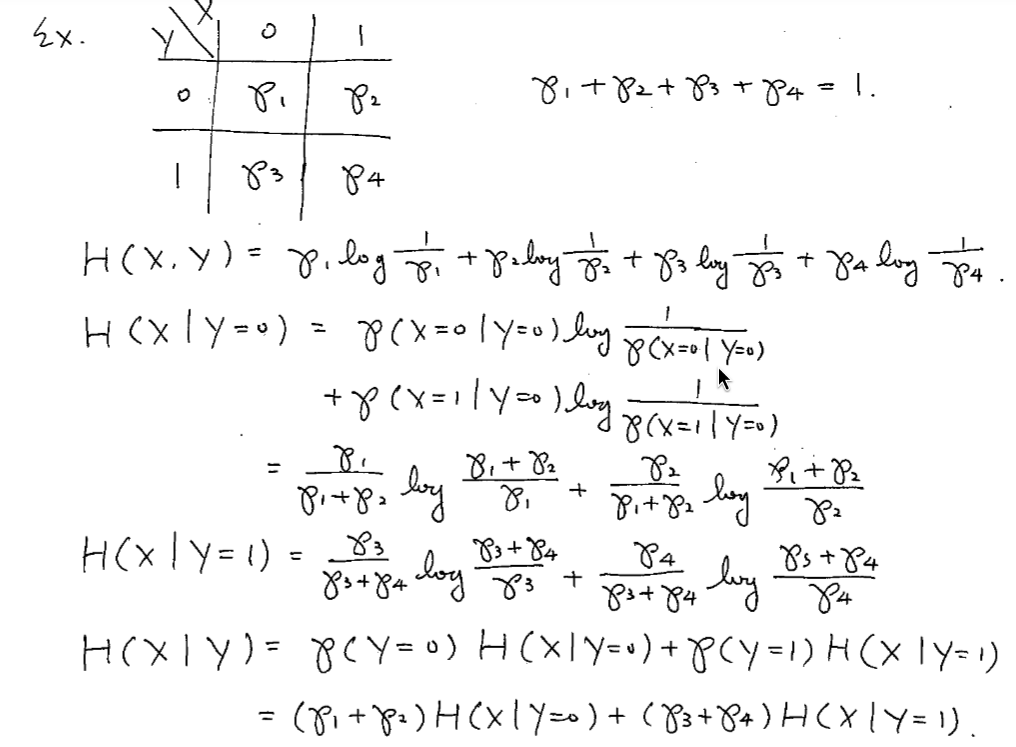
3.2 Properties of $H(X|Y)$
Entropy Chain Rule: $$ H(X, Y) = H(Y) + H(X|Y) $$ Intuition: Total uncertainty of $(X,Y)=$ uncertatinty of $Y$ alone $+$ remaining uncertainty of $X$ after knowing $Y$.
这里的加号可以理解为:熵是信息量,分两步说,第一步先告诉他 $Y$ 是什么,即有 $H(Y)$ 个 bit,第二步是已经知道 $Y$ 的情况下,在告诉他 $X$ 是什么,即 $H(X|Y)$ 个 bit,两步获得的信息量是相加的
By symmetry, $H(X,Y) = H(X) + H(Y|X)$ is also correct.
Extension: Chain rule for joint entropy: $$ H(X_1, X_2, \cdots, X_n) = H(X_1) + H(X_2 | X_1) + H(X_3 | (X_1, X_2)) + \cdots + H(X_n | (X_1, X_2, \cdots X_{n-1})) $$
Theorem: If $X$ and $Y$ are independent (no overlay), then: $$ H(X, Y) = H(X) + H(Y) $$ And we have: $$ H(X|Y) = H(X) \Leftrightarrow X \text{ and } Y \text{ are independent} \\ H(X|Y) = H(Y) \Leftrightarrow X \text{ and } Y \text{ are independent} $$
3.3 Information never hurts
Theorem: Knowing $Y$ will not hurt our existing knowledge of $X$ $$ H(X|Y) \leq H(X) $$
So when in data compression, we can have:
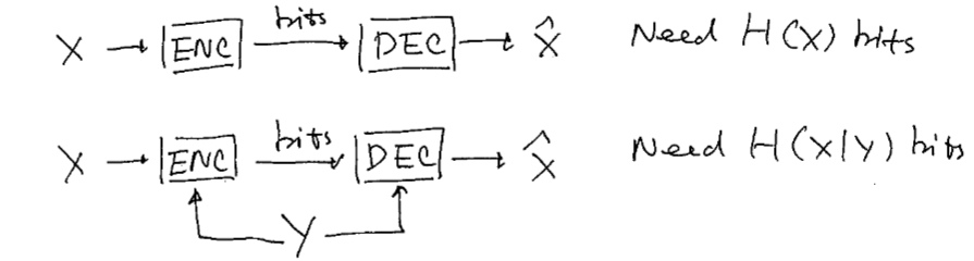
e.g. Consider a probability table.
| $X\backslash Y$ | $0$ | $1$ |
|---|---|---|
| $0$ | $0.45$ | $0.05$ |
| $1$ | $0.05$ | $0.45$ |
And we have $$ X = \begin{cases} 0 \quad 50\% \\ 1 \quad 50\% \end{cases} $$
Without $Y$, we need $H(X) = 1$ bit to describe $X$.
Now $Y$ is provided, we can use the following equations: $$ X \oplus Y = Z \\ Y \oplus Z = X $$ Note that: $$ Z = \begin{cases} 0 \quad 90\% \\ 1 \quad 10\% \end{cases} $$ And we have $H(Z) < H(X)$, so the main idea is compressing $Z$ instead of $X$, and then recover $X$ with XOR.
e.g.
Consider $n$ balls, one ball is odd in that it is lighter or heavier than any other ball. Giving only one balance to compare two balls each time. How many times do we need to figure out which ball is odd?
Chapter 4: Mutual Information
4.1 Basics
Def. Mutual Information $$ \begin{aligned} I(X; Y) &= H(X) - H(X|Y) \\ &= H(X) + H(Y) - H(X, Y) \\ &= \sum_{x, y} p(x, y) \log \frac{p(x,y)}{p(x)p(y)} \\ &= E_{x,y} \left[ \log \frac{p(x,y)}{p(x)p(y)} \right] \\ \end{aligned} $$
Consider X -> Channel -> Y, then $I(X;Y)$ is the maximum number of bits reliably transmitted by our channel.
Now consider the venn graph below:

We have $$ \begin{aligned} &H(X|Y) = A \\ &H(Y|X) = C \\ &I(X;Y) = B \\ &H(X) = A+B \\ &H(Y) = B+C \\ &H(X, Y) = A+B+C \end{aligned} $$
4.2 KL Divergence
Def. For two distributions $p(x), q(x)$, their KL Divergence: $$ D(p || q) = \sum_x p(x) \log \frac{p(x)}{q(x)} $$
$D(p || q)$ gives "distance"(or "difference") between $p$ and $q$. BUT $D(p||q) \not= D(q||p)$
Def. Cross Entropy $$ CE(p,q) = \sum_x p(x) \log \frac{1}{q(x)} $$
Theorem: $$ CE(p,q) = H(p) + D(p||q) $$
CE(交叉熵)其实就是,比如在机器学习中,模型的理解 $q$ 和真实世界 $p$ 差得有多远,真实世界按照 $p$ 产生数据,但我用模型 $q$ 去预测它,平均会有多惊讶(可以作为 loss)
KL Divergence(KL 散度)就是因为用了错误模型 $q$,额外多付出了多少代价
4.3 Hypothesis Testing
Let $X_1, X_2, \cdots, X_n$ be independent random variables, but not sure which is their distribution, $p(x)$ or $q(x)$?
Two hypothesis:
- $H_1: X_i \sim p(x)$
- $H_2: X_i \sim q(x)$
Q: How to use $X_1, X_2, \cdots, X_n$ to decide which is true?
A: If $p(x)$ is more likely to produce $X_1, X_2, \cdots, X_n$, then $H_1$ is true, otherwise $H_2$ is true.
Def. Log-likelihood Ratoi: $$ LLR = \frac{1}{n} \log \frac{p(x_1, x_2, \cdots, x_n)}{q(x_1, x_2, \cdots, x_n)} $$ So the hypothesis test is:
- If $LLR > 0$, $p(x)$ will be the distribution
- If $LLR < 0$, $q(x)$ will be the distribution
Chapter 5: Conditional Mutual Information
5.1 Basics
Def. For $(X,Y,Z) \sim p(x,y,z)$, the conditional mutual information is $$ I(X;Y|Z)=H(X|Z)-H(X|Y,Z). $$
Equivalent forms: $$ \begin{aligned} I(X;Y|Z) &=H(Y|Z)-H(Y|X,Z) \\ &=H(X|Z)+H(Y|Z)-H(X,Y|Z) \\ &=H(X,Z)+H(Y,Z)-H(Z)-H(X,Y,Z). \end{aligned} $$
Interpretation:
- $H(X|Z)$: uncertainty of $X$ after side information $Z$ is known.
- $I(X;Y|Z)$: additional information about $X$ learned from $Y$ after $Z$ is already known.
先知道 $Z$,再看 $Y$。$I(X;Y|Z)$ 问的是:在已经知道 $Z$ 的情况下,$Y$ 还能额外告诉我们多少关于 $X$ 的信息。
Theorem: $$ I(X;Y|Z)\geq 0. $$ Equality holds iff $X$ and $Y$ are conditionally independent given $Z$: $$ p(x,y|z)=p(x|z)p(y|z). $$
Important warning: $$ I(X;Y|Z) $$ can be larger or smaller than $I(X;Y)$.
Example intuition:
- If $Z$ is pure noise independent of everything, conditioning on $Z$ does not help much.
- If $Z$ helps remove noise from $Y$, then $I(X;Y|Z)$ can become larger.
- If $Z$ already reveals $X$, then $I(X;Y|Z)=0$.
5.2 Chain Rule for Mutual Information
Theorem: $$ I(X_1,\cdots,X_n;Y) =I(X_1;Y)+I(X_2;Y|X_1)+\cdots+I(X_n;Y|X_1,\cdots,X_{n-1}). $$
Interpretation:
Instead of decoding all users together, we may decode one by one:
$$ (X_1,\cdots,X_n)\rightarrow \text{Channel}\rightarrow Y. $$
First decode $X_1$, then subtract the known part from $Y$, then decode $X_2$, and so on.
总信息量可以拆成“第一层信息 + 已知第一层后的第二层信息 + 已知前两层后的第三层信息 + ...”。
5.3 Markov Chain and Data Processing
Def. $X\to Y\to Z$ is a Markov chain if $$ p(x,y,z)=p(x)p(y|x)p(z|y). $$
Equivalently, $$ p(z|x,y)=p(z|y). $$
Intuition:
$$ X\to Y\to Z $$ means $Z$ depends on $X$ only through $Y$.
Theorem: If $X\to Y\to Z$, then $Z\to Y\to X$ is also a Markov chain.
Theorem: If $X\to Y\to Z$, then $X$ and $Z$ are conditionally independent given $Y$: $$ I(X;Z|Y)=0. $$
Theorem (Data Processing Inequality): If $$ X\to Y\to Z, $$ then $$ I(X;Z)\leq I(X;Y). $$
Also, $$ I(X;Z)\leq I(Y;Z). $$
信息经过处理不会凭空变多。$X$ 先告诉 $Y$,$Y$ 再告诉 $Z$,所以 $Z$ 对 $X$ 的了解不可能超过 $Y$ 对 $X$ 的了解。
Useful identity for proof: $$ I(X;Y,Z)=I(X;Z)+I(X;Y|Z) =I(X;Y)+I(X;Z|Y). $$
For Markov chain $X\to Y\to Z$, since $I(X;Z|Y)=0$, $$ I(X;Z)+I(X;Y|Z)=I(X;Y). $$
Chapter 6: Three-Party Mutual Information
6.1 Basics
Def. For $(X,Y,Z)\sim p(x,y,z)$, the three-party mutual information is $$ I(X;Y;Z)=I(X;Y)-I(X;Y|Z). $$
Equivalent forms: $$ \begin{aligned} I(X;Y;Z) &=H(X)+H(Y)+H(Z) \\ &\quad -H(X,Y)-H(X,Z)-H(Y,Z)+H(X,Y,Z). \end{aligned} $$
Symmetric identities: $$ I(X;Y;Z)=I(X;Z)-I(X;Z|Y)=I(Y;Z)-I(Y;Z|X). $$
Important warning: $$ I(X;Y)\geq 0,\qquad I(X;Y|Z)\geq 0, $$ but $$ I(X;Y;Z) $$ can be positive, zero, or negative.
two-party MI 和 conditional MI 都不会负;three-party MI 不一样,它不是一个普通的“信息量”,而更像三者重叠关系的代数量。
6.2 Information Theoretic Security
Let
- $X$ be plaintext,
- $K$ be key,
- $Y$ be ciphertext.
Encryption: $$ Y=f(X,K). $$
Decryption: $$ \hat X=g(Y,K). $$
Def. A system has perfect secrecy if $$ I(X;Y)=0. $$
This means the ciphertext reveals nothing about the plaintext without the key.
Def. The system is perfectly decodable if $$ H(X|Y,K)=0. $$
This means once both $Y$ and $K$ are known, $X$ can be recovered exactly.
Example (One-Time Pad):
Let $$ X\sim \operatorname{Bern}\left(\frac12\right),\qquad K\sim \operatorname{Bern}\left(\frac12\right) $$ independently, and define $$ Y=X\oplus K. $$
Then $$ \hat X=Y\oplus K. $$
So $$ I(X;Y)=0,\qquad H(X|Y,K)=0. $$
Theorem (Shannon's Perfect Secrecy Limit): If $$ I(X;Y)=0 $$ and $$ H(X|Y,K)=0, $$ then $$ H(K)\geq H(X). $$
想做到完全安全,key 的不确定性至少要和 message 一样大。One-time pad 安全,但 key 必须和 plaintext 一样长,所以实际很不方便。
Chapter 7: Entropy Rate
7.1 Motivation
For iid random variables $X_1,\cdots,X_n$, $$ H(X_1,\cdots,X_n)=\sum_{i=1}^n H(X_i)=nH(X_1). $$
But natural language, music, text, etc. are not iid. Later symbols depend on previous symbols.
Def. For a stochastic process $\mathcal X={X_i}$, the entropy rate is $$ H(\mathcal X)=\lim_{n\to\infty}\frac1n H(X_1,\cdots,X_n), $$ if the limit exists.
Examples:
If $X_i$ are iid, then $$ H(\mathcal X)=H(X_1). $$
If $X_i=X_1$ for all $i$, then $$ H(\mathcal X)=\lim_{n\to\infty}\frac1n H(X_1)=0. $$
entropy rate 是“平均每个新符号还带来多少新信息”。如果后面全是重复,平均新信息趋近于 0。
7.2 Stationary Stochastic Process
Def. A stochastic process $\mathcal X={X_i}$ is stationary if shifting time does not change the joint distribution: $$ p(X_1,\cdots,X_n)=p(X_{1+k},\cdots,X_{n+k}) $$ for all $n,k$.
Theorem:
For stationary $\mathcal X={X_i}$, $$ \lim_{n\to\infty} H(X_n|X_1,\cdots,X_{n-1}) $$ exists.
Moreover, $$ H(\mathcal X) =\lim_{n\to\infty}\frac1n H(X_1,\cdots,X_n) =\lim_{n\to\infty}H(X_n|X_1,\cdots,X_{n-1}). $$
Key idea:
Let $$ a_n=H(X_n|X_1,\cdots,X_{n-1}). $$
For stationary processes, $a_n$ is non-increasing: $$ a_{n+1}\leq a_n. $$
Also, $$ H(X_1,\cdots,X_n)=\sum_{i=1}^n a_i. $$
So the average converges to the same limit.
7.3 Markov Process
Def. A stochastic process is Markov if $$ p(X_n|X_1,\cdots,X_{n-1})=p(X_n|X_{n-1}). $$
That is, the future depends on the past only through the present.
Theorem:
If $\mathcal X$ is stationary and Markov, then $$ H(\mathcal X)=H(X_2|X_1). $$
If the stationary distribution is $\pi_i$ and transition matrix is $P_{ij}$, then $$ H(\mathcal X) =\sum_i \pi_i H(P_{i,\cdot}) =-\sum_i\sum_j \pi_i P_{ij}\log P_{ij}. $$
Example:
If $$ X_{n+1}=aX_n+Z_n, $$ where $Z_n$ are iid and independent of the past, then $$ H(\mathcal X)=H(X_2|X_1)=H(Z_1). $$
给定 $X_n$ 后,$X_{n+1}$ 的不确定性只来自新的 noise $Z_n$。
Chapter 8: AEP
8.1 LLN and AEP
Theorem (Law of Large Numbers):
For iid $X_i\sim p(x)$, $$ \frac1n\sum_{i=1}^n X_i \to E[X] $$ in probability.
Theorem (Asymptotic Equipartition Property, AEP):
For iid $X_i\sim p(x)$, $$ -\frac1n\log p(X_1,\cdots,X_n)\to H(X) $$ in probability.
Proof idea: $$ p(X_1,\cdots,X_n)=\prod_{i=1}^n p(X_i), $$ so $$ -\frac1n\log p(X_1,\cdots,X_n) =\frac1n\sum_{i=1}^n \log\frac1{p(X_i)}. $$
By LLN, this converges to $$ E\left[\log\frac1{p(X)}\right]=H(X). $$
长序列的概率通常差不多是 $2^{-nH(X)}$。所以虽然每个具体序列概率不同,但“大多数概率质量”集中在一批概率差不多的序列上。
8.2 Typical Set
Def. For $\epsilon>0$, a sequence $(x_1,\cdots,x_n)$ is $\epsilon$-typical if $$ \left|-\frac1n\log p(x_1,\cdots,x_n)-H(X)\right|\leq \epsilon. $$
Def. The typical set is $$ A_\epsilon^{(n)} =\left\{x^n: \left|-\frac1n\log p(x^n)-H(X)\right|\leq \epsilon \right\}. $$
For any $x^n\in A_\epsilon^{(n)}$, $$ 2^{-n[H(X)+\epsilon]} \leq p(x^n)\leq 2^{-n[H(X)-\epsilon]}. $$
Theorem:
For any $\delta>0$, for sufficiently large $n$, $$ \Pr\{X^n\in A_\epsilon^{(n)}\}>1-\delta. $$
Theorem (Size of Typical Set):
For any $\delta>0$, for sufficiently large $n$, $$ (1-\delta)2^{n[H(X)-\epsilon]} \leq |A_\epsilon^{(n)}| \leq 2^{n[H(X)+\epsilon]}. $$
Therefore, $$ |A_\epsilon^{(n)}|\approx 2^{nH(X)}. $$
typical set 的大小远小于全集 $|\mathcal X|^n$,但它包含几乎全部概率质量。压缩就是只给 typical set 里的序列编号。
Example (Binary Source):
If $$ X_i=\begin{cases} 0,&p,\\ 1,&1-p, \end{cases} $$ then a typical sequence contains about $np$ zeros and $n(1-p)$ ones.
Number of typical sequences is roughly $$ \binom{n}{np}\approx 2^{nH(X)}. $$
Important warning:
Typical sequence is not necessarily the most likely sequence.
If $p=0.1$, the most likely sequence may be all $1$'s, but a typical sequence has about $10%$ zeros and $90%$ ones.
8.3 Fundamental Limit of Data Compression
Theorem (Achievability):
For iid $X_i\sim p(x)$ and any $\delta>0$, for sufficiently large $n$, the sequence $$ (X_1,\cdots,X_n) $$ can be described using $$ n[H(X)+\delta] $$ bits with probability of error going to $0$.
Main idea:
- If $x^n\in A_\epsilon^{(n)}$, encode its index inside the typical set.
- This needs about $$ \log |A_\epsilon^{(n)}|\approx nH(X) $$ bits.
- If $x^n\notin A_\epsilon^{(n)}$, use a fallback code.
Theorem (Converse):
There is no set $B_n$ with $$ \Pr\{X^n\in B_n\}\to 1 $$ and $$ |B_n|<2^{n[H(X)-\epsilon]} $$ for large $n$.
$H(X)$ 不是某种“推荐压缩率”,而是极限。高于它可以做到,低于它基本不可能。
Chapter 9: Data Compression
9.1 Variable Length Code
Def. A variable length code is a map $$ c:\mathcal X\to \{0,1\}^* $$ that assigns each source symbol a bit string.
For a sequence, $$ c(x_1,\cdots,x_n)=c(x_1)c(x_2)\cdots c(x_n). $$
Def. A code is uniquely decodable (U.D.) if no two different source sequences produce the same encoded bit string.
That is, $$ (x_1,\cdots,x_n)\neq (y_1,\cdots,y_m) \Rightarrow c(x_1,\cdots,x_n)\neq c(y_1,\cdots,y_m). $$
单个 codeword 不同还不够,因为拼起来以后可能撞车。U.D. 要求任意长串拼接后也不能歧义。
9.2 Prefix-Free Code
Def. A code is prefix-free if no codeword is a prefix of another codeword.
Theorem: $$ \text{prefix-free}\Rightarrow \text{uniquely decodable}. $$
But $$ \text{uniquely decodable}\nRightarrow \text{prefix-free}. $$
Example:
$$ {0,10,110,111} $$ is prefix-free.
Prefix-free codes can be represented by leaves of a binary tree.
9.3 Kraft's Inequality
Theorem (Kraft Inequality):
Let $\ell_i$ be the codeword length for symbol $i$, where $i=1,\cdots,m$.
There exists a binary prefix-free code with lengths $\ell_i$ iff $$ \sum_{i=1}^m 2^{-\ell_i}\leq 1. $$
Tree interpretation:
- A codeword of length $\ell_i$ occupies $2^{\ell_{\max}-\ell_i}$ leaves in a full binary tree of depth $\ell_{\max}$.
- Total occupied leaves cannot exceed $2^{\ell_{\max}}$.
For $D$-ary codes: $$ \sum_{i=1}^m D^{-\ell_i}\leq 1. $$
9.4 McMillan's Inequality
Theorem (McMillan Inequality):
There exists a binary uniquely decodable code with lengths $\ell_i$ iff $$ \sum_{i=1}^m 2^{-\ell_i}\leq 1. $$
For $D$-ary uniquely decodable codes: $$ \sum_{i=1}^m D^{-\ell_i}\leq 1. $$
prefix-free 看起来比 U.D. 更严格,但从“可实现的长度集合”角度看,它们满足同一个 Kraft/McMillan 条件。所以优化平均长度时可以专心找 prefix-free code。
Chapter 10: Shannon Code
10.1 Optimizing Codeword Length
For source alphabet $$ \mathcal X={1,\cdots,m}, $$ suppose symbol $i$ has probability $p_i$ and codeword length $\ell_i$.
We want to minimize expected length: $$ L=\sum_i p_i\ell_i $$ subject to $$ \sum_i 2^{-\ell_i}\leq 1,\qquad \ell_i\in \mathbb Z^+. $$
Relax the integer constraint. The optimal real-valued length is $$ \ell_i^*=\log\frac1{p_i}. $$
Then $$ L^*=\sum_i p_i\log\frac1{p_i}=H(X). $$
Therefore, for any uniquely decodable code, $$ L\geq H(X). $$
概率大的符号应该给短码,概率小的符号给长码。最理想长度就是 surprise:$\log(1/p_i)$。
10.2 Shannon Code
Def. The Shannon code chooses $$ \ell_i=\left\lceil \log\frac1{p_i}\right\rceil. $$
Since $$ \ell_i<\log\frac1{p_i}+1, $$ we have $$ L=\sum_i p_i\ell_i <\sum_i p_i\left(\log\frac1{p_i}+1\right) =H(X)+1. $$
Theorem:
For Shannon code, $$ H(X)\leq L < H(X)+1. $$
If every $p_i$ is a power of $2$, then $\log(1/p_i)$ is integer and $$ L=H(X). $$
10.3 Block Coding
The $+1$ bit overhead may be large for single symbols.
Idea: group $n$ symbols together: $$ Y=(X_1,\cdots,X_n). $$
Design Shannon code for $Y$.
If $X_i$ are iid, then $$ H(Y)=H(X_1,\cdots,X_n)=nH(X). $$
For the block code, $$ H(Y)\leq L_Y < H(Y)+1. $$
Divide by $n$: $$ H(X)\leq \frac{L_Y}{n}<H(X)+\frac1n. $$
As $n\to\infty$, $$ \frac{L_Y}{n}\to H(X). $$
把很多 symbols 打包一起编码,可以把每个 symbol 平均多出来的 overhead 从 $1$ bit 降到 $1/n$ bit。但代价是 codebook size 指数爆炸。
10.4 Wrong Distribution
Suppose the true test distribution is $q_i$, but the code is designed using training distribution $p_i$.
Shannon code length: $$ \ell_i=\left\lceil \log\frac1{p_i}\right\rceil. $$
Expected length under true distribution $q$: $$ \begin{aligned} L &=\sum_i q_i\ell_i \\ &<\sum_i q_i\log\frac1{p_i}+1 \\ &=H(q)+D(q||p)+1 \\ &=CE(q,p)+1. \end{aligned} $$
Note:
- $D(q||p)$ is the extra cost of not knowing the true distribution.
- If $p=q$, then $D(q||p)=0$.
10.5 Value of Side Information
Suppose $(X,Y)$ are correlated, and $Y$ is provided to both encoder and decoder as side information.
For each possible $y$, design a code for $X$ based on $$ p(x|y). $$
For each $y$, $$ H(X|Y=y)\leq L_y < H(X|Y=y)+1. $$
Average over $y$: $$ H(X|Y)\leq L < H(X|Y)+1. $$
Since $$ H(X|Y)\leq H(X), $$ side information can reduce the required number of bits.
如果 decoder 和 encoder 都知道 $Y$,我们可以根据不同的 $Y=y$ 使用不同 codebook。相关性越强,$H(X|Y)$ 越小,越省 bits。
Chapter 11: Huffman Code
11.1 Optimal Solution
Recall the codeword length problem: $$ \min \sum_i p_i\ell_i $$ subject to $$ \sum_i 2^{-\ell_i}\leq 1,\qquad \ell_i\in\mathbb Z^+. $$
Shannon code is simple but may be suboptimal because it only rounds $$ \log\frac1{p_i}. $$
The optimal prefix-free code is given by Huffman coding.
Algorithm (Binary Huffman Code):
- Sort symbols by probability.
- Merge the two least likely symbols.
- Replace them by one combined symbol with probability equal to their sum.
- Repeat until only one symbol remains.
- Assign $0/1$ labels to branches and read codewords from root to leaves.
Expected length: $$ L=\sum_i p_i\ell_i. $$
11.2 Optimality Lemmas
Lemma 1:
For an optimal prefix-free code, if $$ p_i>p_j, $$ then $$ \ell_i\leq \ell_j. $$
More likely symbols should not have longer codewords.
Lemma 2:
In an optimal binary prefix-free code, the two longest codewords can be chosen to have the same length and share the same parent node.
Lemma 3:
In an optimal binary prefix-free code, the two least likely symbols can be assigned to these two longest sibling codewords.
Theorem (Huffman Optimality):
Merging the two least likely symbols reduces the problem to a smaller optimal coding problem.
If the Huffman tree is optimal for the reduced source, expanding the merged node gives an optimal tree for the original source.
Huffman 的贪心是对的,因为在某个最优树里,最小的两个概率一定可以被放在最深处当 siblings。先把它们合并不会破坏最优性。
11.3 Remarks
Huffman code is not unique.
Reasons:
- Ties in probability can be merged in different orders.
- Left/right branches can swap $0$ and $1$.
- Different trees may have the same expected length.
Theorem:
For binary Huffman code, $$ H(X)\leq L_{\text{Huffman}}<H(X)+1. $$
The lower bound follows from entropy being the fundamental limit.
To make $$ L_{\text{Huffman}}\to H(X), $$ we can Huffman-code blocks $$ (X_1,\cdots,X_n), $$ but the codebook size grows exponentially.
11.4 D-ary Huffman Code
For $D$-ary codewords: $$ c:\mathcal X\to \{0,1,\cdots,D-1\}^*. $$
Algorithm:
Merge the $D$ least likely symbols each time.
Important:
For a full $D$-ary tree, the number of leaves must satisfy $$ m\equiv 1 \pmod{D-1}. $$
If not, add dummy symbols with probability $0$ until $$ m+r\equiv 1 \pmod{D-1}. $$
Then run the normal $D$-ary Huffman algorithm.
For $D$-ary code measured in $D$-ary digits, $$ H_D(X)\leq L_D < H_D(X)+1, $$ where $$ H_D(X)=\sum_i p_i\log_D\frac1{p_i}. $$
Measured in bits: $$ H(X)\leq L_D\log_2D < H(X)+\log_2D. $$
Midterm Cheat-Sheet Priority
Must memorize:
$$ H(X,Y)=H(X)+H(Y|X) $$
$$ I(X;Y)=H(X)-H(X|Y)=H(X)+H(Y)-H(X,Y) $$
$$ I(X;Y|Z)=H(X|Z)-H(X|Y,Z) $$
$$ D(p||q)=\sum_x p(x)\log\frac{p(x)}{q(x)}\geq 0 $$
$$ A_\epsilon^{(n)}\approx 2^{nH(X)},\qquad p(x^n)\approx 2^{-nH(X)} $$
$$ \sum_i 2^{-\ell_i}\leq 1 $$
$$ H(X)\leq L_{\text{Shannon}},L_{\text{Huffman}}<H(X)+1 $$
Most likely exam operations:
- Expand entropy / mutual information expressions.
- Prove inequalities using chain rule and "conditioning reduces entropy".
- Compute typical set size or probability.
- Compute entropy rate for stationary Markov processes.
- Construct Huffman code and compute expected length.
MAT3007 Optimization
Prof. Yongchun Li
Three main subjects:
- Linear Optimization
- Disciplined linear programming
- Algorithms
- Duality
- Nonlinear Optimization
- Optimally condition
- Nonlinear optimization alorigthms
- Integer Optimization
- Baisc algorithms
- Assignments: 30%
- Midterm Exam(24 June): 30%
- Final Exam(18 July): 40%
Lecture 1
Brief Introduction
Common components of optimization problems:
- Decision 决策
- Objective 目标
- Constraints 限制条件
Optimization concerns choosing a decision(or decisions) to optimize certain objectives while subject to certain constraints.
最优化即选择一个决策(或一些决策)去最优化一些目标,在某些限制条件下。
Optimize could mean maximize or minimize depending on the problem contxt. 最大化 / 最小化
Optimization Problems
Mathematically, an optimization problem is usually represented as: $$ \begin{aligned} \min_{x} \quad & f(x) \\ \text{subject to} \quad & x \in \Omega \end{aligned} $$ where we have $x$ for Decision, $f$ for Objective funtion and $\Omega$ for Constraints.
In practice, we often consider a slightly more restrictive form: $$ \begin{aligned} \min_{x \in R^n} \quad & f(x) \\ \text{subject to } \quad & g_i(x) \leq 0, \quad \forall i = 1, \cdots, m \\ \text{subject to } \quad & h_j(x) = 0, \quad \forall i = 1, \cdots, p. \end{aligned} $$ where $x \in R^n$ is Decision variables(a vector), $f(x)$ is Objecive funtion and $g(x) \leq 0, h(x) = 0$ is Inequality and equality constraints. $$ g(x) = \begin{bmatrix} g_1(x) \\ \vdots \\ g_m(x) \end{bmatrix} \in R^m \text{ and } h(x) = \begin{bmatrix} h_1(x) \\ \vdots \\ h_p(x) \end{bmatrix} \in R^p $$ We can also express the constraints using the abstarct format: $$ \begin{aligned} \Omega &:= \{x \in R^n: g_i(x) \leq 0, i = 1, \dots, m, h_j(x) = 0, j = 1, \dots, p \} \\ &= \{x \in R^n: g(x) \leq 0, h(x) = 0 \} \end{aligned} $$
Feasible point: A decition that satisfies all constraints. 可行点
Feasible region(set) $\Omega$: The set of all feasible points.
Optimal solution:
Optimal value
Minimizer 最优解
Let $\Omega \subseteq R^n$ be a nonempty set and let $f : \Omega \to R$ be given. We define $$ B_{\epsilon(y)} := \{x \in R^n: \Vert x-y \Vert < \epsilon \} $$ to be the open ball(开球) in $R^n$ with center $y$ and radius $\epsilon > 0$
The point $x^* \in R^n$ is said to be a:
- Local minimizer(局部最优解)
- Strict local minimizer(严格局部最优解)
- Global minizer(全局最优解)
- Strict global minimzer(严格全局最优解)
Remark: global minimizer = global solution = optimal solution
Properties of Optimization Problems
Some facts:
- The feasible set can be empty(infeasible).
- An optimization problem may not always have an optimal solution.
- The optimal value can be unbounded.
- Even if an opt. problem is feasible, finite, and can attain its optimal value, the optimal solution may not be unique.
By classifying the different outcomes, an opt. problem may have the following stats:
- Infeasible
- Feasible, optimal value finite but not attainble.
- Feasible, optimal value finite and attainable.
- Feasible, but optimal value is unbounded.
Classifications of Optimization
Unconstrained optimization: If $m = p = 0$. Otherwise constrained optimization.
Linear Programming(LP): Constraints and objective function are linear in the decision variables.
Nonlinear Programming(NLP): Either some of the constraints or the objective funtion if nonlinear.
Convex Optimization: If $f(x)$ and all $g_i(x)$ and convex, and $h_j(x)$ are linear (i.e. the feasible set is convex).
Integer Programming(IP): Some of the decision variables have to be integers.
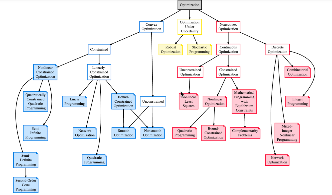
Modeling 建模
e.g. Maximum Area Problem.
You have 80 meters of fencing and want to enclose a rectangular area - as large as possible.
- Decision variable: the length $l$ and width $w$ of the area.
- Objective: maximize the area: $lw$
- Constraints: the total length of the fence: $2l + 2w \leq 80$
Therefore, the optimization problem can be written as $$ \begin{aligned} \max_{l, w} \quad & lw \\ \text{subject to} \quad & 2l+2w \leq 80 \ & l, w \geq 0 \end{aligned} $$
e.g. Shortest Path Problem
Set of notdes $V$, set of edges: $E \subset V \times V$. The distance between node $i$ and node $j$ is $w_{ij}$.
For each edge $(i, j) \in E$, define $$ x_{ij} = \begin{cases} 1 , & \text{if we use edge }(i,j), \\ 0 , & \text{otherwise}. \end{cases} $$
Directed graph: $x_{ij}$ does not necessarily equal to $x_{ji}$. And we have the following optimization modeling
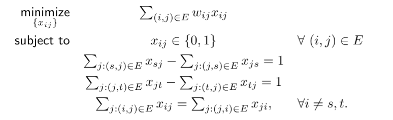
Lecture 2
Linear Programming 线性规划
Def. A linear optimization or linear programming(LP) problem is an optimization problem in which the objective function and all constraint functions are linear (in the decision variables)
e.g. $$ \begin{aligned} \max_{x_1, x_2, x_3} \quad & f(x) = 40 x_1 + 30 x_2 + 50 x_3 \\ \text{subject to} \quad & x_1 + x_2 + x_3 \leq 100 \\ & 2x_1 + x_2 + 3x_3 \leq 180 \\ & x_3 \geq x_1 \\ & x_1, x_2, x_3 \geq 0 \end{aligned} $$
General Formulation
$$ \begin{aligned} \min_{x \in R^n} \quad & c^\top x \\ \text{subject to} \quad & a_i^\top x \geq b_i \quad &\forall i \in m_1 \\ & a_i^\top x \leq d_i \quad &\forall i \in m_2 \\ & a_i^\top x = e_i \quad &\forall i \in m_3 \\ & x_i \geq 0 \quad &\forall i \in n_1 \\ & x_i \leq 0 \quad &\forall i \in n_2 \\ & x_i \text{ free} \quad &\forall i \in n_3 \end{aligned} $$
where $m_1, m_2, m_3$ are subsets of $\{1, \dots, m\}$, $n_1, n_2, n_3$ are subsets of $\{1, \dots, n\}$.
Standard Form of LPs
An LP is said to be of the standard form if it is of the form: $$ \begin{aligned} \min_{x \in R^n} \quad & c^\top x \\ \text{subject to} \quad & Ax = b \\ & x \geq 0 \end{aligned} $$
where $x \in R^n$, $A$ is an $m \times n$ matrix($m < n$), and $b \in R^m$.
Any LP can be written in the standard form, using "tricks".
Standard From Transformations:
- Maximization: use $-c$ instead of $c$ to change it to minimization.
- Eliminating inequality constraints using slack variables $s$.
- $Ax \leq b \Rightarrow Ax+s=b, s \geq 0$
- $Ax \geq b \Rightarrow Ax-s=b, s \geq 0$
- If one has $x_i \leq 0$, replace $x_i$ by $-y_i$ and add $y_i \geq 0$
- Eliminating free variables $x_i$ (no constraints on $x_i$) by replacing $x_i$ by $x_i^+ - x_i^-$, where $x_i^+ \geq 0, x_i^- \geq 0$
e.g.
Consider a LP problem: $$ \begin{aligned} \max \quad & 3x_1 - 2x_2 + x_3 \\ \text{subject to} \quad & 2x_1 + 3x_2 + 4x_3 \geq 1 \\ & 3x_1 + 4x_2 \leq 5 \\ & 5x_2 - x_3 = -1 \\ & x_1, x_2 \geq 0 \end{aligned} $$
We can transform it into standard form: $$ \begin{aligned} \min \quad & -3x_1 + 2x_2 - x_3^+ + x_3^- \\ \text{subject to} \quad & 2x_1 + 3x_2 + 4x_3^+ - 4x_3^- - x_4 = 1 \\ & 3x_1 + 4x_2 + x_5 = 5 \\ & 5x_2 - x_3^+ + x_3^- = -1 \\ & x_1, x_2, x_3^+, x_3^-, x_4, x_5 \geq 0 \end{aligned} $$
More Modeling
Minimax Objective Problem: $$ \begin{aligned} \min_x \quad & \max_{i=1,\cdots,n} \{ c_i^\top x + d_i \} \\ \text{subject to} \quad & Ax=b \\ & x \geq 0 \end{aligned} $$
Solution: define $y = \max_{i=1,\cdots,n} \{ c_i^\top x + d_i \}$ and consider: $$ \begin{aligned} \min_{x,y} \quad & y \\ \text{subject to} \quad & y \geq c_i^\top x + d_i \\ & Ax=b \\ & x \geq 0 \end{aligned} $$
Minimizing Absolute Values $$ \begin{aligned} \min_x \quad & \sum_{i=1}^n \lvert x_i \rvert \\ \text{subject to} \quad & Ax=b \\ \end{aligned} $$ This can be equivalently written as: $$ \begin{aligned} \min_{x,t} \quad & \sum_{i=1}^n t_i \\ \text{subject to} \quad & x_i \leq t_i \\ & x_i \geq -t_i \\ & Ax=b \end{aligned} $$
A Modeling Tool
Consider the optimization problem: $$ \begin{aligned} \min_{x} \quad & \sum_{i=1}^m f_i(x) \\ \text{subject to} \quad & x \in \Omega \end{aligned} $$ It is equivalent to $$ \begin{aligned} \min_{x,t} \quad & \sum_{i=1}^m t_i \\ \text{subject to} \quad & x \in \Omega \\ & f_i(x) \leq t_i \end{aligned} $$ Where $f_i: R^n \to R$ are given and $\Omega \subset R^n$ is the feasible set.
Lecture 3
Solving Linear Programming Graphically
Recall the production problem: $$ \begin{aligned} \max \quad & x_1 + 2x_2 \\ \text{subject to} \quad & x_1 \leq 100 \\ &2x_2 \leq 200 \\ &x_1 + x_2 \leq 150 \\ &x_1, x_2 \geq 0 \end{aligned} $$
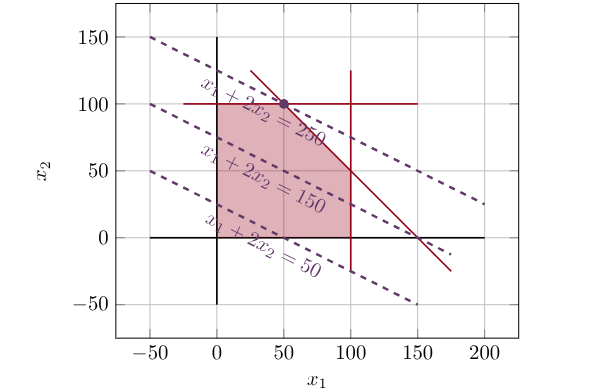
The red polygon is the feasible region.
And the optimal solution is the highest one among these lines that touches the feasible region.
Some Obeservations:
- The feasible region of an LP is a polyhedron 多面体
- The optimal solution tends to be a vertex/corner of the feasible region.
- Some constraints are active at the optimal solution, some are inactive
Def. A Polyhedron is a set that can be written in the form $$ \{ x \in R^n: Ax \geq b \} $$ where $A$ is an $m \times n$ matrix and $b \in R^m$.
注:这里的 Polyhedron 多面体,并不是传统意义上的三维多面体,而是可以有更高维度的多面体,无法直观现象。
Def. Convex Set: A set $S \subseteq R^n$ is convex if $$ \forall x, y \in S \\ \forall \lambda \in [0,1], \lambda x + (1- \lambda) y \in S $$
Def. Convex Combination: For any $x_1, \cdots, x_n$ and $\lambda_1 + \cdots + \lambda_n = 1$, we call $\sum_{i=1}^n \lambda_i x_i$ a convex combination of $x_1, \cdots, x_n$.
Def. Exetreme Point: Let $P$ be a polyhedron. A point $x \in P$ is said to be an extreme point of $P$ if we cannot find two elements $y,z \in P$ with $y,z \not= x$ and a scalar $\lambda \in [0,1]$, such that $x = \lambda y + (1-\lambda) z$.
Consider the production problem example above, it has $5$ exetreme points.
Exetreme Points and Basic Feasible Solutions
Consider an LP in its standard form: $$ \begin{aligned} \min_{x \in R^n} \quad & c^\top x \\ \text{subject to} \quad & Ax = b \\ & x \geq 0 \end{aligned} $$ where $x \in R^n$, $A$ is an $m \times n$ matrix($m < n$), and $b \in R^m$.
General Assumption: $A$ has linearly independent rows (or equivalently $A$ hass full row rank $m$)
Def. Basic Solution: We call $x$ a basic solution(BS) of the standard form LP iff:
- $Ax = b$
- There exist indices $B(1), \cdots, B(m)$ such that the columns of $$ \begin{bmatrix} | & | & & | \\ A_{B(1)} & A_{B(2)} & \cdots & A_{B(m)} \\ | & | & & | \end{bmatrix} $$ are linear independent and $x_i=0$ for $i \not= B(1), \cdots, B(m)$.
Finding a Basic Solution
Procedure:
- Choose any $m$ independent columns of $A$: $A_{B(1)}, \cdots, A_{B(m)}$
- Let $x_i=0$ for all $i \not= B(1), \cdots, B(m)$.
- Solve the equation $Ax=b$ for the remaining $x_{B(1)}, \cdots, x_{B(m)}$, giving $x_B = A_B^{-1} b$
Since $A_{B(1)}, \cdots, A_{B(m)}$ are linearly independent, the last step must produce a unique solution. Basic solution of an LP only depends on its constraints, it has nothing to do with the objective function.
Basic Feasible Solutions
Def. If a basic solution $x$ also satisfies that $x \geq 0$, then we call it a basic feasible solution (BFS).
Example
Still production problem...
$$
\begin{aligned}
\max \quad & x_1 + 2x_2 \\
\text{subject to} \quad & x_1 \leq 100 \\
&2x_2 \leq 200 \\
&x_1 + x_2 \leq 150 \\
&x_1, x_2 \geq 0
\end{aligned}
$$
with standard form:
$$
\begin{array}{rlrrrrrrl}
\min & -x_1 & & -2x_2 & & & & & \\
\text{subject to} & x_1 & & & & +s_1 & & & = 100 \\
& & & 2x_2 & & & & +s_2 & = 200 \\
& x_1 & & +x_2 & & & &+ s_3 & = 150 \\
& x_1, & & x_2, & & s_1, & & s_2, \quad s_3 & \ge 0
\end{array}
$$
We can denote the fesibale set by $\{ x:Ax=b, x \geq 0 \}$ where
$$
A =
\begin{bmatrix}
1 & 0 & 1 & 0 & 0 \\
0 & 2 & 0 & 1 & 0 \\
1 & 1 & 0 & 0 & 1
\end{bmatrix}, \quad
b =
\begin{bmatrix}
100 \\
200 \\
150
\end{bmatrix}
$$
We can choose three independent columns of $A$, e.g. the first three $(B = \{1, 2, 3\})$, we get the corresponding basic solution via:
$$
x_B =
\begin{bmatrix}
1 & 0 & 1 \\
0 & 2 & 0 \\
1 & 1 & 0
\end{bmatrix}^{-1}
\begin{bmatrix}
100 \\
200 \\
150
\end{bmatrix} =
\begin{bmatrix}
50 \\
100 \\
50
\end{bmatrix}
$$
That is $x_1 = 50, x_2 = 100, s_1 = 50$, therefore $(50, 100, 50, 0, 0)$ is a basic feasible solution.
One can find other basic feasible solution by choosing other sets of columns.
Extreme Points and BFS
For the standard LP polyhedron $\{ x:Ax=b, x \geq 0 \}$, we have:
$x$ is an extreme point $\Leftrightarrow$ $x$ is a basic feasible solution.
就是说,我们的可行解可以组成一个多面体,这个多面体的极值点(也就是顶点)其实就是 BFS,即通过组合矩阵 $A$ 里面的列组成满秩矩阵得到的解,作为端点,形成的多面体。
为什么满秩矩阵接出来的解即这个多面体的顶点?本质上可以理解为同时选了几个约束都到了极值点,那自然就形成了可行解的顶点。
Fundamental Theorem of LP
Fundamental LP Theorem: Consider a linear problem in standard form and assume that $A$ has full row rank $m$.
- If the feasible set is nonempty, there is a basic feasible solution.
- If there is an optimal solution, there must be at least one optimal solution that is also a basic feasible solution.
Corollary: Characteristics: If an LP with $m$ constraints (in the standard form) has an optimal solution, then there must be an optimal solution with no more than $m$ positive entries.
Lecture 4
The Simplex Method 单纯形法
Idea: The simplex method preceeds from one BFS (an extreme point of the feasible region) to a neighboring / adjacent one to continuously imporve the value of the object funtion until reaching optimality.
It usually talks on standard form LP: $$ \begin{aligned} \min_{x} \quad & c^\top x \\ \text{subject to} \quad & Ax=b \\ & x \geq 0 \end{aligned} $$
Neighboring BFS
Def. Neighboring Basic Solutions: Two basic solutions are neighboring / adjacent if they differ by exactly one baic (or non-basic) index.
e.g. A BFS constructed by using $B=\{ 1,2,3 \}$ is a neighbor to $B=\{ 1,3,5 \}$, but not a neighbor to $B=\{ 1,4,5 \}$
So if we consider checking all the neighbors of a BFS, which consists $m(n-m)$ potential neighbors, it likely to be very slow.
Finding a Neighboring BFS
First, we assume that we have somehow found a BFS whose basis is $B=\{ B(1),\cdots,B(m) \}$, and define: $$ \begin{bmatrix} | & | & & | \\ A_{B(1)} & A_{B(2)} & \cdots & A_{B(m)} \\ | & | & & | \end{bmatrix} $$ And let $A_N$ be the matrix consisting of the non-basic columns of $A$. We have $$ |B| = m, |N|=n-m \\ B \cup N = \{1,2,\cdots,n\} $$ We can write $$ A=[A_B, A_N], x=[x_B;x_N] $$ By definition, we have $$ x_B = A_B^{-1}b \quad x_N = 0 $$
To find a neighbor, we want to select a non-basic variable $x_j, j \in N$ to enter the basis. Which means we want to increase $x_j$ from the current BFS.
Basic Direction
We consider moving $x$ to a neighboring one $y$ by $$ y=x+\theta d, \quad \theta \geq 0 $$ where
- $d_j=1$
- $d_{j'}=0$ for all other non-basic indices $j' \not= j \in N$.
We need to guarantee that the resulting step $y=x+\theta d$ is still feasible, that is: $$ A(x+\theta d) = b = Ax $$ i.e. $Ad=0$
Now, we write $d=[d_B;d_N]$, since $d_j=1$ and $d_{j'}=0$ for all other non-basic indices, we have $$ 0= \begin{bmatrix} A_B & A_N \end{bmatrix} \begin{bmatrix} d_B \\ d_N \end{bmatrix}= A_B d_B + A_j $$ Therefore $$ d_B = -A_B^{-1}A_j $$ Which means the direction $d$ is uniquely determined once $j$ is chosen: $$ d=[d_B;d_N]=[-A_B^{-1}A_j;0;\dots;1;\dots;0] $$ where the $1$ is at the $j^{th}$ entry, we call such $d$ the $j^{th}$ basic direction.
简单来讲,就是我们现在站在一个 BFS(顶点)上,我们想要走到相邻顶点。我们选一个 non-basic 变量 $x_j$,让它从 $0$ 开始变大,且一直满足 $Ax=b$ 约束。
当 $x_j$ 增加时,basic 变量也必须跟着变化,来抵消 $x_j$ 对约束的影响,,其方向为 $d_B=-A_B^{-1}A_j$。然后沿着 $y=x+\theta d$ 走,直到某个 basic 变量变成 $0$,那这个变成 $0$ 的 basic 变量就会离开 basis。
至此,得到了一个新的 BFS。但是,朝着这个方向走,目标函数会变好吗(更优)?
Reduced Cost
The target function is
$$
c^\top x
$$
if walking $x$ to $y=x+\theta d$, the change of function will be
$$
\begin{aligned}
\Delta &= c^\top y-c^\top x \\
&= c^\top (x+\theta d)-c^\top x\\
&= \theta c^\top d
\end{aligned}
$$
We define the reduced cost
$$
\begin{aligned}
\bar{c}_j &= c^\top d \\
&= c_B^\top d_B + c_j \\
&= c_B^\top (-A_B^{-1}A_j)+c_j \\
&= c_j - c_B^\top A_B^{-1} A_j
\end{aligned}
$$
And in minimization problem, if a non-basic variable $x_j$'s reduced cost satisfies $\bar{c}_j < 0$, it means it will decrease the function (better direction) if it enters basis.
Thus simplex will choose a variable of $\bar{c}_j < 0$ to enter basis.
If all non-basic variables satisfy $\bar{c}_j \ge 0$, it means there is no neibouring that decrease the target function, and it is the Optimization Answer.
Theorem: Stopping Criterion
Consider a basic feasible solution $x$ associated with the basis $B(1), B(2), \cdots, B(m)$ and let $\bar{c} = [\bar{c}_1; \cdots; \bar{c}_n]$ be the corresponding vector of reduced costs. If $\bar{c}_j \ge 0$, then $x$ must be optimal.
这个比较好理解,就是不断找能使得目标函数更小的加入 Basis,顺便带走一个,直到找不到能替换的为止。
Choosing a Stepsize $\theta$
After choosing an entering variable, we know the direction $d$, but we still need to choose how far we can move along this direction while keeping feasibility.
The feasibility requires: $$ y = x + \theta d \ge 0 $$ For variables with $d_i \ge 0$, there is no restriction on $\theta$, but for variables with $d_i < 0$, we need $$ x_i + \theta d_i \ge 0 $$ $$ \theta \le -\frac{x_i}{d_i} $$ Therefore the largest feasible stepsize is: $$ \theta^* = \min_{i\in B, d_i <0} \left\{ -\frac{x_i}{d_i} \right\} $$
其实就是,沿着这个方向 $d$ 走,谁先变成 $0$,谁就限制了能走多远。
Consider the minimum number is reached by a basic variable $x_\ell$, we have $$ \theta^* = -\frac{x_\ell}{d_\ell} $$ $$ y_\ell = x_\ell + \theta^* d_\ell = 0 $$ That is, $x_\ell$ is leaving basis, and the entering variable $x_j$ is entering basis. The basis changed from $B$ to $B'=B-\{\ell\} + \{j\}$.
This is a simplex pivot.
What if no variable is decreasing?
If the direction satisfies $$ d \ge 0 $$ That is walking along the direction and all variables are not gonna be negative. $$ x + \theta d \ge 0 $$ Meanwhile since we are choosing $$ \bar{c}_j < 0 $$ So the target function is always decreasing, that is the LP has no limit optimal solution, which is unbounded.
Conclusion
Initialization: We start from a BFS $x$ with corresponding basis $B$.
-
We first compute the reduced costs $\bar{c}$: $$ \bar{c}_j = c_j - c_B^\top A_B^{-1} A_j $$
- If $\bar{c} \ge 0$, then $x$ is optimal.
- Otherwise choose some $j \in N$ such that $\bar{c} < 0$.
-
Compute the $j^{th}$ basic direction $d$ $$ d = [-A_B^{-1}A_j;0;\cdots;1;\cdots;0] $$
- If $d \ge 0$, then the problem is unbounded.
- Otherwise, compute $\theta^*$:
$$ \theta^* = \min_{i\in B, d_i <0} \left\{ -\frac{x_i}{d_i} \right\} $$
-
Set $y=x+\theta^* d$. Then the point $y$ is the new BFS with index $j$ replacing $B(\ell)$ in the basis. The objective function value (decrease) is changed by $$ \theta^* c^\top d = \theta^* \bar{c}_j $$
-
Repeate this procedures.
站在当前 BFS 上,用 reduced cost 找一个能让目标变好的 non-basic variable,让它进入 basis;然后沿着对应 basic direction 走,用 minimum ratio test 找最多能走多远;走到某个 basic variable 变成 $0$,让它离开 basis;得到新的 BFS;重复直到所有 reduced costs 都不能让目标变好。
Lecture 5
Degeneracy
Def. We call a BFS $x$ degenerate if some of the basic variables $x_B$ are $0$. Otherwise, it is non-degenerate.