CSC4120 Design and Analysis of Algorithms
L0 Introduction
Main Course Topics
- Key algorithm concepts (asymptotic complexity, divide-and-conquer)
- Basic data structure algorithms
- Heaps (priority queues)
- Binary seach trees (scheduling)
- Hashing (cryptography, dictionaries)
- Graph searches (reachability analysis)
- Shortest paths (Google maps, navigation)
- Greedy algorithms (minimum spanning trees, Huffman codes)
- Dynamic programming (any optimization problem)
- Network flows
- Compleity (NP-complete, poly reductions, approximation algorithms)
Textbook: Algorithms by S. Dasgupta, C.H. Papadimitriou, and U.V. Vazirani.
L1 Basic Concepts of Algorithmic Performance
Asymptotic Complexity
What is $T(n)$?
$T(n)$ is the largest (worst) execution time over all inputs of size $n$.
Asymptotic Complexity
Goal: Capture the growth of $T(n)$ of an algorithm as the problem instance size $n \rightarrow \infty$
Key Idea: Keep only the rate of growth, i.e., the dominant term when $n \rightarrow \infty$, forgetting multiplicative constants and lower order terms.
Three Os
-
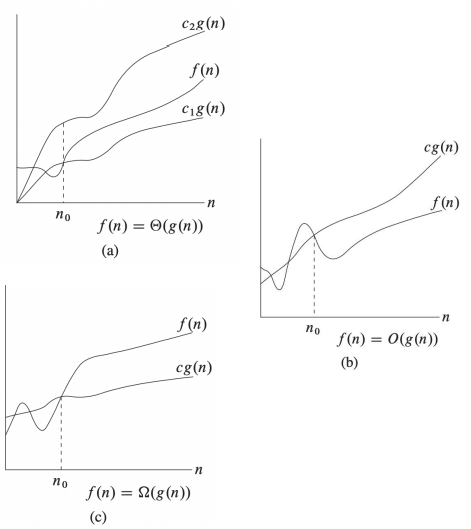
$\Theta$: Grows asymptotically as fast as ($=$)
- Tight Bound
- $f(n) = \Theta(g(n)) \Leftrightarrow \exists c_1, c_2 > 0, n_0 \text{ s.t. } c_1 g(n) \leq f(n) \leq c_2 g(n) \text{ for } n \geq n_0$
- e.g. $100n^2 + 5n - 5 = 0.1n^2 + 10n^{1.5} - 5 = \Theta(n^2)$
-
$O$: Grows asymptotically at most as fast as ($\leq$)
- Upper Bound
- $f(n) = O(g(n)) \Leftrightarrow \exists c > 0, n_0 \text{ s.t. } f(n) \leq c g(n) \text{ for } n \geq n_0$
- e.g. $2n^{1.5}-5 \leq n^{1.5} \leq n^2 \Rightarrow 2n^{1.5}-5 = O(n^{1.5}), = O(n^2)$
- e.g. $n^{1.5} \leq n^2 \leq 2^n \Rightarrow n^{1.5} = O(n^2), n^2 = O(2^n), n^{1.5} = O(2^n)$
-
$\Omega$: Grows asymptotically at least as fast as ($\geq$)
- Lower Bound
- $f(n) = \Omega(g(n)) \Leftrightarrow \exists c > 0, n_0 \text{ s.t. } f(n) \geq c g(n) \text{ for } n \geq n_0$
- e.g. $5 \leq 2n \leq n^{1.5}+1 \leq 2^n \Rightarrow 2n = \Omega(1), 2^n = \Omega(n^{1.5})$
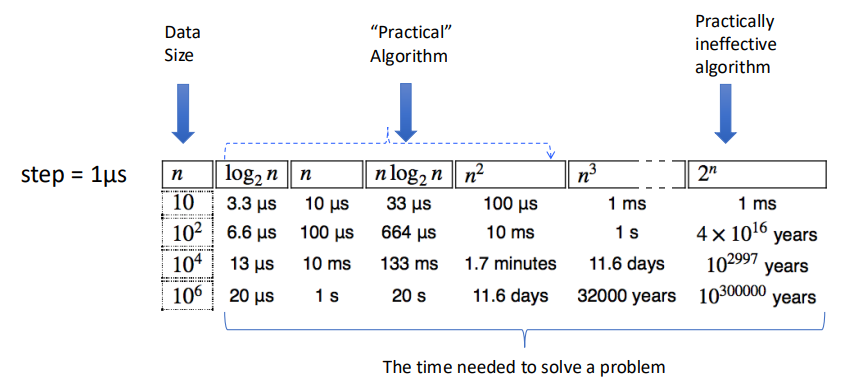
In Practice
Conclusions
- To measure the performance of algorithms we measure their asymptotic complexity.
- Big $O$ is used to describe an upper bound for the running time of an algorithm.
- Big $\Omega$ is used to describe a lower bound for the running time of an algorithm.
- Big $\Theta$ is used to denote asymptotic equivalence of the running times of two algorithms. And when $\Omega(g(n)) = O(g(n)) = f(n)$, we can have $\Theta(g(n)) = f(n)$
L2 Divide and Conquer
Divide and Conquer (Sorting and Master Theorem)
Basic Devide and Conquer
There are 3 steps:
- Divide input into multiple smaller (usually disjoint) points.
- Conquer each of the parts separatelly (using recursive calls).
- Combine results from different calls.
$$ T(n) = \text{divide time} \\ +T(n_1) + T(n_2) + \cdots + T(n_k) \\ +\text{combine time} $$
Sorting
A non-D&C solution: Insertion Sort
void insertionSort(int arr[], int n) {
    for (int i = 1; i < n; i++) {
        int key = arr[i];
        int j = i - 1;
        while (j >= 0 && arr[j] > key) {
            arr[j + 1] = arr[j];
            j--;
        }
        arr[j + 1] = key;
    }
}
We have the complexity is $O(n^2)$ since it runs two loops with $n$ steps.
But $O(n^2)$ is too slow for most of the problem, can it be much faster? Of course. We can use divide and conquer here!
A D&C solution: Merge Sort
void merge(vector<int>& arr, int l, int m, int r) {
    int n1 = m - l + 1;
    int n2 = r - m;
    vector<int> L(n1), R(n2);
    for (int i = 0; i < n1; i++) L[i] = arr[l + i];
    for (int j = 0; j < n2; j++) R[j] = arr[m + 1 + j];
    int i = 0, j = 0, k = l;
    while (i < n1 && j < n2) {
        if (L[i] <= R[j]) arr[k++] = L[i++];
        else arr[k++] = R[j++];
    }
    while (i < n1) arr[k++] = L[i++];
    while (j < n2) arr[k++] = R[j++];
}

void mergeSort(vector<int>& arr, int l, int r) {
    if (l < r) {
        int m = l + (r - l) / 2;
        mergeSort(arr, l, m);
        mergeSort(arr, m + 1, r);
        merge(arr, l, m, r);
    }
}
From the function mergeSort we can see that we divide the array into $2$ parts and conquer them seperately and recursively. And the merge function has the time complexity of $\Theta(n)$.
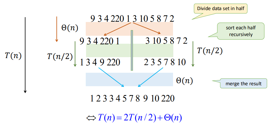
From the graph we can see that there is only $\log n$ levels of recursion. Thus, we have
$$ \begin{align*} T(n) &= 2T(n/2) + cn \\ &= (cn) \log n + nT(1) \\ &= \Theta (n \log n) \end{align*} $$
Where $cn$ denotes for the time of divide and merge, and $T(1)$ represents for the node of the recursion tree.
Geometric Sums
Consider a geometric series $$ S = 1 + x + x^2 + \cdots + x^h = \frac{x^{x+1}-1}{x-1} \ \ (\text{for } x \not= 1) $$ If $x < 1$, then $$ 1 + x + x^2 + \cdots + x^h \in \left[ 1, \frac{1}{1-x} \right] \Rightarrow S = \Theta(1) $$ If $x > 1$ , then $$ 1 + x + x^2 + \cdots + x^h < \frac{1}{1-x} x^h \Rightarrow S = \Theta(x^h) $$
Master Theorem
Consider the recursion:
$$ T(n) = aT(n/b) + f(n) $$
- Number of levels: $\log_b n = \Theta(\log n)$
- Number of leaves: $L = a^{\log_b n} = n^{log_b a}$
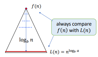
We use the recursion tree to calculate the cost. The cost of the $i$-th (root $i=0$) is: $$ \begin{align*} C_i &= (\text{Nodes Number of } i \text{-th Level}) \times (f \text{ of Every Subproblem}) \\ &= a^i f(n/b^i) \end{align*} $$ So that, we have: $$ T(n) = \sum_{i=0}^h C_i = \sum_{i=0}^{\log_b n} a^i f(n/b^i) $$
We need to compare the time within root and leaves to get the main factor. The usual method is to compare $f(n)$ and $L(n) = n^{\log_b a}$
There are 3 situations here:
-
Geometrically Increasing (Leaves): $$ f(n) = O(L^{1-\epsilon}) \Rightarrow T(n) = \Theta(L) $$ e.g. $T(n) = 2T(n/2) + \sqrt{n}$, we have $a=2, b=2, L=n^{\log_b a} = n$, and $\sqrt{n} = n^{1/2} = O(L^{1-\epsilon})$, thus $T(n) = \Theta(n)$
-
Roughly Equal Levels: $$ f(n) = \Theta(L) \Rightarrow T(n) = \Theta (L \log n) \\ f(n) = \Theta(L \log n) \Rightarrow T(n) = \Theta (L \log^2 n) $$ e.g. $T(n) = 2T(n/2) + n$, we have $L=n^{\log_2 2} = n$, and $n = O(L)$, thus $T(n) = \Theta(n \log n)$
-
Geometrically Decreasing (Root) + Regularly Condition $$ f(n) = \Omega(L^{1+\epsilon}) \text{ and } af(n/b) \leq sf(n), s < 1 \Rightarrow T(n) = \Theta(f(n)) $$ e.g. $T(n) = 2T(n/2) + n^2$, we have $L=n^{\log_2 2} = n$, and $n^2 > O(L), 2f(n/2) = 2(n/2)^2 \leq (1/2) f(n)$, thus $T(n) = \Theta(n^2)$
Applications of D&C
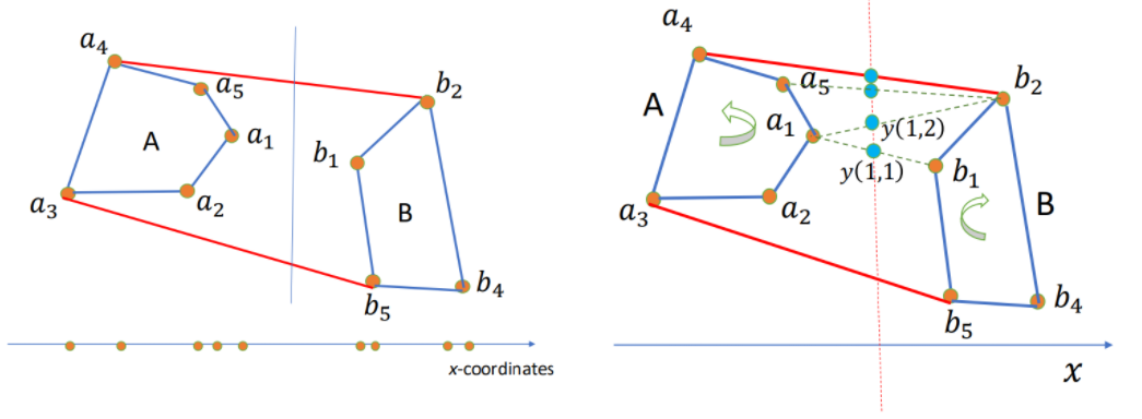
Convex Hull
Given $n$ points $S = { (x_i, y_i) | i = 1, 2, \cdots, n }$ s.t. all have different $x$ and $y$ coordinates, and no three of them in a line.
Convex Hull (CH): The smallest polygon containing all points in $S$. Represented by the sequence of points in the boundary in clockwise order.
How to use D&C here?
- Sort points by $x$-coordinate.
- For our input set $S$ of points:
- Divide (by $x$-coordinates) into left-half A and right-half B.
- Compute CH(A) and CH(B).
- Merge CH(A) and CH(B) to get CH(A+B).
It has the complexity time $T(n) = 2T(n/2) + \Theta(n) \rightarrow \Theta(n \log n)$.
BUT, how to merge?
Algorithm: Start with $(a_1, b_1)$. While $y(i, j)$ increases, keep moving by one step either a_i counterclockwise or b_j clockwise. When cannot increase anymore, we found the upper tangent, say $a_u, b_u$. Similarly, the lower tangent $a_l, b_l$. Then the CH = points of A clockwise from $a_l$ to $a_u$ + points of B clockwise from $b_u$ + $b_l$. Hence total time $\Theta(n)$
Median Finding / Peak Finding
Not interested.
Fast Fourier Transform
Multiplication of polynomials as list of coefficients.
Consider: $$ \begin{align*} A(x) &= a_0 + a_1 x + \cdots + a_n x^n = \sum_{i=0}^{n}a_i x^i \\ B(x) &= b_0 + b_1 x + \cdots + b_n x^n = \sum_{i=0}^{n}b_i x^i \end{align*} $$ To calculate: $$ \begin{align*} C(x) &= A(x) B(x) = c_0 + c_1 x + \cdots + c_{2n}x^{2n} =\sum_{i=0}^{2n}c_i x^i \\ \text{where }c_k &= a_0 b_k + a_1 b_{k-1} + \cdots + a_k b_0 = \sum_{i=0}^k a_i b_{k-i} \end{align*} $$
Complexity: For $c_k \rightarrow O(k)$, for $C(x) \rightarrow O(n^2)$
Can we do it faster? Like $O(n \log n)$?
Multiplication of polynomials as list of values.
Consider: A degree-$n$ polynomial is uniquely characterized by its values at any $n+1$ distinct points $x_0, x_1, \cdots, x_d$.
That is, if we fix any distinct $n+1$ points, we can specify any degree-$n$ polynomial $A(x) = a_0 + a_1 x + \cdots + a_d x^n$ by the $n+1$ values: $$ A(x_0), A(x_1), \cdots, A(x_n) $$ Then we can have: $$ \begin{align*} C(x) &= A(x) B(x) \\ C(x_i) &= A(x_i) B(x_i) \\ \text{where } i&=0,1,\cdots,2n \end{align*} $$ Polynomial multiplication is $O(n)$ using this representation!
But how can we get the coefficients of $C(x)$ ?
Evaluation and Interpolation
Evaluation: $a_0, a_1, \cdots, a_n \rightarrow A(x_0), A(x_1), \cdots, A(x_n)$
$$ A(x) = M_n(x) \cdot a \\ $$ $$ \begin{bmatrix} A(x_0) \\ A(x_1) \\ \vdots \\ A(x_{n}) \end{bmatrix}= \begin{bmatrix} 1 & x_0 & x_0^2 & \cdots & x_0^n \\ 1 & x_1 & x_1^2 & \cdots & x_1^n \\ \vdots & \vdots & \vdots & \ddots & \vdots \\ 1 & x_n & x_n^2 & \cdots & x_n^n \end{bmatrix} \cdot \begin{bmatrix} a_0 \\ a_1 \\ \vdots \\ a_{n} \end{bmatrix} $$
Interpolation: $A(x_0), A(x_1), \cdots, A(x_n) \rightarrow a_0, a_1, \cdots, a_n$ $$ a = M_n^{-1}(x) \cdot A(x) \\ $$ $$ \begin{bmatrix} a_0 \\ a_1 \\ \vdots \\ a_n \end{bmatrix}= \begin{bmatrix} 1 & x_0 & x_0^2 & \cdots & x_0^n \\ 1 & x_1 & x_1^2 & \cdots & x_1^n \\ \vdots & \vdots & \vdots & \ddots & \vdots \\ 1 & x_n & x_n^2 & \cdots & x_n^n \end{bmatrix} ^{-1} \cdot \begin{bmatrix} A(x_0) \\ A(x_1) \\ \vdots \\ A(x_n) \end{bmatrix} $$
Here $M_n$ is Vandermonde matrix.
Consider $C(x_i) = A(x_i) B(x_i)$, from the two matrix multiplication we can know that: If we have every $A(x_i)$ and $B(x_i)$ we can use $O(n)$ to multiply and get $C(x_i)$, then transfer it into every coefficient $c_i$.
But, using matrix multiplication directly will need time complexity of $O(n^2)$. Can we optimize it to $O(n \log n)$? Yes, and here comes Fast Fourier Tranform (FFT).
FFT
Let's calculate evaluation using FFT first.
Consider a polynomial $P(x)$ with length of even number $n$ s.t. $$ \begin{align*} P(x) &= a_0 + a_1 x + a_2 x^2 + \cdots + a_{n-1} x^{n-1} \\ &= P_{\text{even}}(x^2) + x \cdot P_{\text{odd}}(x^2) \\ \text{where } P_{\text{even}}(x) &= a_0 + a_2 x + a_4 x^2 + \cdots + a_{n-2} x^{n/2} \\ P_{\text{odd}}(x) &= a_1 + a_3 x + a_5 x^2 + \cdots + a_{n-1} x^{n/2} \end{align*} $$
By doing this, we divide the the length $n$ to two length $n/2$. Then, we have to conquer them each and then combine them together.
Let $A_k$ denote $A(x_k)$.
The question is: How can we divide $A_k$?
And here's the most essencial part: We use primitive root $\omega$.
Now, think about an complex equation: $$ z^n = (re^{i\theta})^n = 1 $$ We can get the solutions: $$ \begin{align*} r &= 1 \\ \theta &= \frac{2k\pi}{n} \\ \text{where } k &= 0, 1, \cdots, n-1 \end{align*} $$ Thus, $$ \begin{align*} \omega_n &= e^{\frac{2\pi}{n}i} \\ \omega_n^k &= e^{\frac{2\pi}{n}ki} = e^{i\theta} \\ (\omega_n^k)^n &= 1 \end{align*} $$ To each $k$, we want to calculate: $$ \begin{align*} A_k &= P(\omega_n^k) \\ &= P_{\text{even}}(\omega_n^{2k}) + \omega_n^k \cdot P_{\text{odd}}(\omega_n^{2k}) \\ &= P_{\text{even}}(\omega_{n/2}^{k}) + \omega_n^k \cdot P_{\text{odd}}(\omega_{n/2}^{k}) \end{align*} $$ Since $$ \omega_n^{2k} = e^{\frac{2\pi}{n} 2ki} = e^{\frac{2\pi}{n/2} ki} = \omega_{n/2}^k $$ This is called the Discrete Fourier Tranform (DFT) of $A_k$.
And we found that: $$ \begin{align*} A_{k+n/2} &= P(\omega_n^{k+n/2}) \\ &= P_{\text{even}}(\omega_{n/2}^{k+n/2}) + \omega_n^{k+n/2} \cdot P_{\text{odd}}(\omega_{n/2}^{k+n/2}) \\ &= P_{\text{even}}(\omega_{n/2}^{k} \cdot \omega_{n/2}^{n/2}) + \omega_n^k \cdot \omega_n^{n/2} \cdot P_{\text{odd}}(\omega_{n/2}^{k} \cdot \omega_{n/2}^{n/2}) \\ &= P_{\text{even}}(\omega_{n/2}^{k}) - \omega_n^k \cdot P_{\text{odd}}(\omega_{n/2}^{k}) \end{align*} $$ Since $$ \omega_n^n = e^{\frac{2\pi}{n}ni} = e^{2\pi i} = 1 \\ \omega_n^{n/2} = e^{\frac{2\pi}{n} (n/2)i} = e^{\pi i} = -1 $$
Combining $A_k$ and $A_{k+n/2}$ together for $0 \leq k < n/2$, we can do D&C here! Since $P_{\text{even}}(\omega_{n/2}^{k})$ and $P_{\text{odd}}(\omega_{n/2}^{k})$ can calculate from the half DFT.
The time complexity is $T(n) = 2T(n/2) + O(n) = O(n \log n)$. We get the whole evaluation.
IFFT
To do interpolation, we need Inverse Fast Fourier Tranfrom (IFFT).
Inverse FFT is easy to explain using Linear Algebra.
It's easy since: $$ a = M_n^{-1}(\omega) \cdot A(\omega) = \frac{1}{n} M_n(\omega^{-1}) \cdot A(\omega) $$ And it's over.
Let $A(\omega) = \text{FFT}(a, \omega)$, then $a = \frac{1}{n} \text{FFT}(A, \omega^{-1})$.
The Whole Progress
- Filled $A(x)$ and $B(x)$ to length of $n=2^k$ by $0$ due to easier FFT D&C.
- Calculate $A(\omega^k)$ and $B(\omega^k)$ for each $k=0,1,\cdots,n-1$, where $\omega = e^{\frac{2\pi}{n}i}$ using FFT.
- Calculate $C(\omega^k) = A(\omega^k) \cdot B(\omega^k)$.
- Calculate $c_i$ using IFFT.
L3 Randomized Algorithms
Basic Concepts of Randomized Algoirthms
Randomized Algorithms: On the same input, different executions of the same algorithm may result in different running times and different outputs.
Type of polynomial randomized algorithms:
- Monte Carlo: Bounded number of steps, but might not find the answer.
- Runs in polynomial time, $P_r$(answer is correct)$=p_o > \frac{1}{2}$.
- Always able to check the answer for correctness.
- How to use: Repeat if neccessary, use majority of answers.
- Las Vegas: No guarantee on max number of steps, always finds answer.
- Runs in expected polynomial time.
- Not stop until finds the correct answer.
$\overline{T}(n)$: Expected time to terminate for a given input of size $n$.
Quicksort
Consider combining D&C and randomize
- Pick an pivot $x$ of the array.
- Divide: Partition the array into subarrays using $x$.
- Conquer: Recursively sort $A$, $B$.
- Combine: $A$, $x$, $B$.
$\overline{T}(n) = \Theta(n \log n)$ for all inputs. $\Rightarrow$ Random selection of $x$ makes no input to be worse.
Or we can say $\Theta(n \log n)$ is the average complexity of quicksort.
Frievald's Algorithm
Given $n \times n$ matrices $A$, $B$ and $C$, check that $AB = C$ (yes or no).
It's very slow to use brute force algorithm since matrices multiplication is $O(n^3)$.
Consider randomization (Frievald's Algorithm):
- Choose a random binary vector $r$.
- If $(A(Br) = Cr) \bmod 2$ then output "yes" else "no".
Property: If $AB \not= C$, then $\text{Pr}[A(Br) \not= Cr] \geq \frac{1}{2}$.
That is, Do 10 tests, if all say "yes", the probability of error $< \left( \frac{1}{2} \right)^{10}$.
L4 Lower Bounds and Heaps
Comparison Model
Comparsion Sort
All the sorting algorithms we've seen so far are comparison sort (merge sort, insertion sort, bubble sort, etc.).
And the best running time that we've seen for comparison sort is $O(n \log n)$. Is it the best we can do?
Decision-Tree
A given recipe for sorting $n$ numbers $a_1, a_2, \cdots, a_n$.
Nodes are suggested comparisons: $i, j$ means compare $a_i$ to $a_j$ for $i, j \in \{1, 2, \cdots, n\}$
The figure below is an example of decision-tree of sorting $a_1 = 9, a_2 = 4, a_3 = 6$.
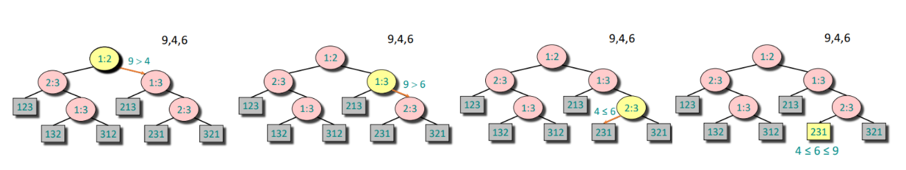
From the tree we can see that:
- A path from the root to the leaves of the tree represents a trace of comparisons that the algorithm may perform.
- The running time of the algorithm = the length of the path taken.
- Worst-case running time = height(depth) of tree
The tree must contain $\geq n!$ leaves since there are $n!$ possible permutations. And a height-$h$ binary tree has $L_h \leq 2^h$ leaves.
Hence: $$ n! \leq L_h \leq 2^h \iff h > \log(n!) \iff h = \Omega(n \log n) $$
Since the Stirling's approximation: $$ n! \approx \sqrt{2 \pi n} \left(\frac{n}{e}\right)^n \\ \log(n!) = n \log n - n + \frac{1}{2} \log (2 \pi n) $$
Theorem: Any decision tree that can sort $n$ elements must have height $\Omega(n \log n)$.
Linear Time Sorting
As metioned above, the comparison sorting have a lower-bound complexity of $\Omega(n \log n)$, so do linear time sorting exist?
Counting Sort
Given: An array $a_0, a_1, \cdots, a_{n-1}$ of $n$ keys to be sorted.
Count the times of number appeared between $a_{min}$ and $a_{max}$, then use the prefix sum array to get the final place of each element. With time complexity of $O(n+k), k = a_{max} - a_{min} + 1$
void counting_sort(vector<int>& a) {
    int n = a.size();
    int mn = *min_element(a.begin(), a.end());
    int mx = *max_element(a.begin(), a.end());
    int k = mx - mn + 1;
    vector<int> count(k, 0);
    for (int x : a) count[x - mn]++;
    for (int i = 1; i < k; i++) count[i] += count[i - 1];
    vector<int> res(n);
    for (int i = n - 1; i >= 0; i--) {
        int x = a[i];
        res[--count[x - mn]] = x;
    }
    a = res;
}
Radix Sort
Use a radix(base) $k$ for an integer $x$: $$ x = a_{d-1} k^{d-1} + \cdots + a_0 k^0 \to a_{d-1}a_{d-2}\cdots a_0 $$
Idea: Sort on least-significant digit first with auxiliary stable sort.
We are given $n$ integers, each integer $< M$, in base $k$. Then we have time complexity of $O((n+k) \log_k M)d$
Heaps
Storing Objects in Data Structures
We operate on objects of the form: object $x = (x.\text{key}, x.\text{data})$.
The attribute $x.\text{key}$ characterizes uniquely the object $x$. And we store $x.\text{key}$ combined with a pointer to the location of $x.\text{data}$ in memory.
Inserting and searching for object $x$ is done by inserting and searching for $x.\text{key}$. Or we can say we mostly focus on $x.\text{key}$ instead of $x.\text{data}$.
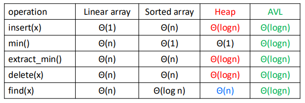
Priority Queue
$S$: set of elements $\{ x_1, x_2, \cdots, x_n \}$.
$x_i = (\text{key}_i, \text{data}_i)$.
Operations: $\text{Insert}(S,x), \max(S), \text{Extract-max}(S), \text{Incr-key}(S, x, k)$.
Heap
Heap: An array visualized as a nearly complete binary tree.
Navigate on the tree but move on array = full info of the tree, without pointers.
Max(Min) Heap Property: the key of a node is $\geq (\leq)$ than the keys of its children.
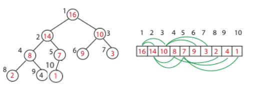
Binary Tree Structure in array, as shown above.
int s[MAXN], sz;

int parent(int i) {
    return i >> 1; // i/2
}

int left(int i) {
    return i << 1; // i*2
}

int right(int i) {
    return i << 1 | 1; // i*2+1
}
And the height of the tree is $h = \log n$.
Max Heapify: Correct a single violation of the heap property occurring at the root $i$ of a subtree in $O(\log n)$.
void max_heapify(int i) {
    int l = left(i), r = right(i), maxi = i;
    if(l <= sz && s[l] > s[maxi]) maxi = l;
    if(r <= sz && s[r] > s[maxi]) maxi = r;
    if(maxi != i) {
        swap(s[i], s[maxi]);
        max_heapify(maxi);
    }
}
Build Max Heap: Convert an array $A$ into a max heap. And we find that elements from $A_{\lfloor n/2 \rfloor+1}$ to $A_n$ are leaves of the tree, and they won't violate the rule. So we only need to heapify $A_1$ to $A_{\lfloor n/2 \rfloor}$. The time complexity is $O(n)$.
void build_max_heap(int n) {
    sz = n;
    for(int i = n/2; i >= 1; i--) max_heapify(i);
}
Insert: We first put it at the back of the array, then go up in the tree one level by one level until no violation.
void insert(int val) {
    sz++;
    s[sz] = val;
    int i = sz;
    while(i > 1 && s[parent(i)] < s[i]) {
        swap(s[i], s[parent(i)]);
        i = parent(i);
    }
}
Extract Max: The max element must be the first one of the array, we can just swap it with the last element, then heapify.
int extract_max() {
    if(!sz) return -1;
    int maxn = s[1];
    s[1] = s[sz];
    sz--;
    max_heapify(1);
    return maxn;
}
Heap Sort: Like extracting max element for $n$ times. Time complexity $O(n \log n)$.
void heap_sort() {
    int n = sz;
    for(int i = n; i >= 2; i--) {
        swap(s[1], s[i]);
        sz--;
        max_heapify(1);
    }
}
L5 Trees
Binary Search Tree
A Binary Search Tree(BST) is a binary tree structure that every node $x$ of it must satisfies:
- All $\text{key}$ from its left subtree is less than $x.\text{key}$
- All $\text{key}$ from its right subtree is greater than $x.\text{key}$
And we can easily know that the left subtree and right subtree of $x$ are both BST.
Define Node: Using C++ struct and pointers.
struct node {
    int key;
    node* left;
    node* right;
    node(int k): key(k), left(NULL), right(NULL) {}
};
Insert: Start from the root, if the $\text{key}$ is less, put it to the left, else to the right. Doing the whole progress in recursion, until find an empty place and put it in. With average time complexity $O(\log n)$, but worst $O(n)$.
node* insert(node* root, int key) {
    if(!root) return new node(key);
    if(key < root->key) {
        root->left = insert(root->left, key);
    } else if(key > root->key) {
        root->right = insert(root->right, key);
    }
    return root;
}
Build Tree: Actually there's no such a thing, you just need to insert the new node into root.
node* root = NULL;
root = insert(root, a);
Inorder Traversal: The inorder traversal of the BST is a sorted array, due to the property of it.
void printTree(node* root) {
    if(!root) return;
    printTree(root->left);
    cout << root->key << " ";
    printTree(root->right);
}
Search: Tipical binary search on tree.
node* search(node* root, int key) {
    if(!root || root->key == key) {
        return root;
    }
    if(key < root->key) {
        return search(root->left, key);
    } else {
        return search(root->right, key);
    }
}
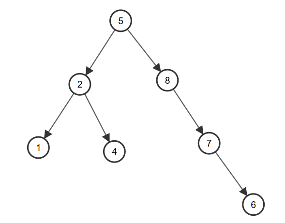
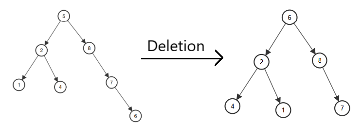
Delete: A bit complicated.
- Leaf (no children): Delete directly.
- On child: Use the child to replace it.
- Two children: Find the minimum of right subtree, replace it with the element we want to delete, and delete it.
node* deleteNode(node* root, int key) {
    if(!root) return NULL;

    if(key < root->key)
        root->left = deleteNode(root->left, key);
    else if(key > root->key)
        root->right = deleteNode(root->right, key);
    else {
        if(!root->left && !root->right) {
            delete root;
            return NULL;
        } else if(!root->left) {
            node* temp = root->right;
            delete root;
            return temp;
        } else if(!root->right) {
            node* temp = root->left;
            delete root;
            return temp;
        } else {
            node* temp = findMin(root->right);
            root->key = temp->key;
            root->right = deleteNode(root->right, temp->key);
        }
    }
    return root;
}
Warning: We usually use the different key to insert, but if there exists two same keys, we can do a count, or change the right subtree to greater or equal subtree.
AVL Tree
An AVL (Adelson-Velskii and Landis) Tree is a self-balancing binary search tree.
Property: For every node, store its height:
- Leaves have height $0$
- NIL has height $-1$
Invariant: For every node $x$, the heights of its left child and right child differ by at most $1$.
And we can know that AVL trees always have height $\Theta(\log n)$.
Define Node: Like BST, but with height.
struct node {
    int key, height;
    node* left;
    node* right;
    node(int k): key(k), height(1), left(NULL), right(NULL) {}
};
Get Height: For convenience, I take leaves height as $1$, NIL height as $0$.
int getHeight(node* u) {
    return u ? u->height : 0;
}
Get Balance: Use the definition of balance, $\text{BL} = \text{height}(\text{left subtree}) - \text{height}(\text{right subtree})$, notice that if $\text{BL} > 1$, left subtree is heavy, else if $\text{BL} < 1$, right subtree is heavy, else it's balanced at this node.
int getBalance(node* u) {
    return u ? getHeight(u->left) - getHeight(u->right) : 0;
}
Right Rotate:
      A                 B
     / \               / \
    B   T3    ->      T1  A
   / \                   / \
  T1  T2                T2  T3
node* rightRotate(node* u) {
    node* v = u->left;
    node* w = v->right;
    v->right = u;
    u->left = w;
    u->height = max(getHeight(u->left), getHeight(u->right)) + 1;
    v->height = max(getHeight(v->left), getHeight(v->right)) + 1;
    return v;
}
Left Rotate:
    A                      B
   / \                    / \
  T1  B        ->        A   T3
     / \                / \
    T2  T3             T1  T2
node* leftRotate(node* u) {
    node* v = u->right;
    node* w = v->left;
    v->left = u;
    u->right = w;
    u->height = max(getHeight(u->left), getHeight(u->right)) + 1;
    v->height = max(getHeight(v->left), getHeight(v->right)) + 1;
    return v;
}
Insert: Consider insertion with 4 situations (L and R means insert into left and right subtree):
- LL: Do right rotation once.
- RR: Do left rotation once.
- LR: Do left rotation, then right rotation.
- RL: Do right rotation, then left rotation.
node *insert(node* u, int key) {
    if(!u) return new node(key);
    if(key < u->key) u->left = insert(u->left, key);
    else if(key > u->key) u->right = insert(u->right, key);
    else return u;
    u->height = max(getHeight(u->left), getHeight(u->right)) + 1;
    int BL = getBalance(u);
    if(BL > 1 && key < u->left->key) return rightRotate(u); // LL
    if(BL < -1 && key > u->right->key) return leftRotate(u); // RR
    if(BL > 1 && key > u->left->key) { // LR
        u->left = leftRotate(u->left);
        return rightRotate(u);
    }
    if(BL < -1 && key < u->right->key) { // RL
        u->right = rightRotate(u->right);
        return leftRotate(u);
    }
    return u;
}

Delete: As same as deletion in BST, then check whether it's balanced.
node* findMin(node* u) {
    while(u->left) u = u->left;
    return u;
}

node* deleteNode(node* u, int key) {
    // BST Deletion first
    if(!u) return NULL;
    if(key < u->key) u->left = deleteNode(u->left, key);
    else if(key > u->key) u->right = deleteNode(u->right, key);
    else {
        if(!u->left || !u->right) {
            node* temp = u->left ? u->left : u->right;
            if(!temp) {
                temp = u;
                u = NULL;
            } else {
                *u = *temp;
            }
            delete temp;
        } else {
            node* temp = findMin(u->right);
            u->key = temp->key;
            u->right = deleteNode(u->right, temp->key);
        }
    }
    if(!u) return NULL;
    // Keep balance
    u->height = max(getHeight(u->left), getHeight(u->right)) + 1;
    int BL = getBalance(u);
    if(BL > 1 && getBalance(u->left) >= 0)
        return rightRotate(u); // LL
    if(BL > 1 && getBalance(u->left) < 0) {
        u->left = leftRotate(u->left);
        return rightRotate(u); // LR
    }
    if(BL < -1 && getBalance(u->right) <= 0)
        return leftRotate(u); // RR
    if(BL < -1 && getBalance(u->right) > 0) {
        u->right = rightRotate(u->right);
        return leftRotate(u); // RL
    }
    return u;
}
Time Complexity: In balanced BST, all operations take $O(\log n)$.
Red-Black Tree
Shit.
Interval Tree
Interval Tree is a balanced BST but nodes are intervals.
Define Node: Interval has $l$ and $r$, while $\text{maxn}$ is the maximum $r$ of all interval of the whole subtree, and we use $l$ as the $\text{key}$ of BST.
struct interval {
    int l, r;
};

struct node {
    interval i;
    int maxn;
    node* left;
    node* right;
    node(interval in): i(in), maxn(in.r), left(NULL), right(NULL) {}
};
Insert: Like regular BST, using $l$ as the $\text{key}$, and record $\text{maxn}$.
node* insert(node* u, interval i) {
    if(!u) return new node(i);
    if(i.l < u->i.l) u->left = insert(u->left, i);
    else u->right = insert(u->right, i);
    u->maxn = max(u->maxn, i.r);
    return u;
}
Search: To get all the intervals who are overlapping with $i$, there are 3 situations
- If the node has overlap with $i$, record the answer.
- If its left subtree's $\text{maxn}$ is greater than $i.l$, search in the left subtree.
- If the node's $l$ is less than $i.r$, search in the right subtree.
bool isOverlap(interval a, interval b) {
    return a.l <= b.r && a.r >= b.l;
}

void searchAll(node* u, interval i, vector<interval>& re) {
    if(!u) return;
    if(isOverlap(u->i, i)) re.push_back(u->i);
    if(u->left && u->left->maxn >= i.l) searchAll(u->left, i, re);
    if(u->right && u->i.l <= i.r) searchAll(u->right, i, re);
}
The regular Interval Tree is like BST with worst time complexity $O(n)$ for each operation, but it can be optimized by AVL tree or other balanced tree, reducing the time complexity to $O(\log n)$.
vEB Tree
An vEB (van Emde Boas) Tree is a data structure that can support below functions in a integer set $S \subseteq \{ 0, 1, \cdots, U-1 \}$, while $U$ is the range of integers (e.g. $U=2^{16}$)
L6 Hashing
Basic Concepts of Hashing
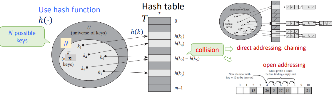
Hash Function: A function that maps data of arbitrary size to fixed-sized values. And the goal is to propose a data structure such that for key $k$:
- $\text{add}(k), \text{delete}(k) = O(1)$
- $\text{search}(k) = O(1)$ on the average
From what I've learnt, the most important thing is not the precise hashing function itself, but the critical thought of hashing.
Hash Table: A table that stores indice and values of hashing.
Making Choices
Choosing the Keys:
- By Nature: Randomly from $U$. (Simple uniform hashing)
- By an Opponent: That knows the hash function we use when this is fixed, in a way to create the longest possbile chain. (Universal hashing)
Choosing the Hash Funcions:
- We use a fixed hash function everyone knows.
- We change before each experiments the hash function, chosen randomly from a "universal set" of functions known to everyone.
Special Case (perfect hashing): We know the keys, then choose the hash function.
Performance: Average length of chain in a typical slot (same hashing value).
Models for Randomness
Simple Uniform Hashing Assumption (SUHA)
$h$ is fixed: In every experiment each key $k$'s value is chosen randomly (uniformly) from $U$.
- Then, $h$ is "good" if $h(k)$ scatters uniformly over the hash table: $$ P_k[h(k) = i] = \frac{1}{m}, \forall i = 1, 2, \cdots, m $$
- We call this the Simple Uniform Hashing Assumption.
Universal Hashing
The set of keys to be stored is assumed fixed: In every experiment, $h$ is randomly (uniformly) chosen from a set $H$.
- Then, $H$ is "good" if $$ P_h[h(k_1) = h(k_2)] \leq \frac{1}{m}, \forall k_1 \not= k_2 $$
- $H$ is a set of Universal Hash Funcions
Actually, Universal Hashing is not a hash function, but designing a set of hash functions. It will randomly choose a hash function when using. Or we can san Universal Hashing is using SUHA by randomization, in order to decrese the probability of collisions.
Universal Hashing Function Examples
The Matrix Method
Settings:
- Keys are $u$-bits long, $|U| = 2^u$
- Hash values are $b$-bits long, hash table size $m = 2^b$
And we pick $h = $ random $b \times u$ $0/1$ matrix, define: $$ h(x) = h \cdot x \pmod 2 $$
Which means matrix multiplication under module $2$.
Claim: For $x \not= y, P_h[h(x) = h(y)] \leq \frac{1}{m} = \frac{1}{2^b}$
e.g. $$ x = 2 = \begin{bmatrix} 1 \\ 0 \\ 1 \\ 0 \end{bmatrix}, h = \begin{bmatrix} 1 & 0 & 0 & 0 \\ 0 & 1 & 1 & 1 \\ 1 & 1 & 1 & 0 \end{bmatrix} $$ And we get $$ h(x) = h \cdot x = \begin{bmatrix} 1 \\ 1 \\ 0 \end{bmatrix} = 6 $$
Linear Hashing for Vector Keys
Settings:
- Suppose keys are vectors $x = (x_1, x_2, x_3, x_4)$, where $x_i$ is an $8$-bit integer. (i.e. $0 \leq x \leq 255$)
- We use a hash table of size $m = p$, where $p$ is a prime number slightly greater than $255$ (e.g. $257$).
Choose the vector of coefficients $a = (a_1, a_2, a_3, a_4)$ where $a_i$ is (uniformly) randomly selected in the range $\{0, 1, \cdots, m-1\}$ And we define: $$ h_a(x) = \left( \sum_{i=1}^4 a_i x_i \right) \bmod m $$
So the hash family is $$ H = \{ h_a : a \in [0, m-1]^4 \} $$
Claim: For $x \not= y, P_a[h_a(x) = h_a(y)] = \frac{1}{m}$
Affine Hashing for Integer Keys
Also called the Carter-Wegman construction
Settings:
- Keys are integers $k \in U$
- Pick a prime number $p$ s.t. $|U| \leq p \leq 2|U|$
- Table size $m \leq p$
We radomly choose $a \in \{ 1, 2, \cdots, p-1 \}, b \in \{ 0, 1, \cdots, p-1 \}$, and define: $$ h_{a,b}(k) = ((a \cdot k + b) \bmod p) \bmod m $$
Claim: For $x \not= y, P_{a,b}[h_{a,b}(x) = h_{a,b}(y)] \leq \frac{1}{m}$
e.g. $|U| = 2^4 = 16, p = 17, m = 6, k = 8, a = 3, b = 4$, then: $$ h_{3,4}(8) = ((3 \cdot 8 + 4) \bmod 17) \bmod 6 = 5 $$
Rolling Hash
Sliding window, but in hashing.
Rabin-Karp Algorithm
Consider a string $S = s_0 s_1 s_2 \cdots s_{n-1}$. We define a window of length $k$ s.t. $T = s_i s_{i+1} \cdots s_{i+k-1}$. And we use the polynomial hash function: $$ H_i = H(T) = (s_i \cdot p^{k-1} + s_{i+1} p^{k-2} + \cdots + s_{i+k-1} \cdot p^0) \bmod M $$ Where $p$ is the base, $M$ is a large prime number and $s_i$ is the ASCII number.
From the function above we can get: $$ H_{i+1} = ((H_i - s_i \cdot p^{k-1}) \cdot p + s_{i+k}) \bmod M $$
And then we can $O(1)$ check whether a string of length $k$ is appeared in $S$.
Table Doubling
We define Load Factor: $$ \alpha = \frac{n}{m} $$ Where $n$ is the element number in hash table, $m$ is the bucket number of hash table.
We have known that we need a hash table to store the keys and values, but if the element number in table is too large, it will cause more and more collisions, which slowing down the hashing progress.
So if $\alpha$ is too large (usually $1$), we will double the bucket number $m$, then rehash all the elements into new table.
Average Cost of Insertions $=\frac{2^{i+2}c + 2^i c_0}{2^i} = O(1)$
Or observe that up to any time $t$: by paying $O(1)$ per insert, covers at all times the total actual cost. We say that insert has an amortized cost of $O(1)$.
Perfect Hashing
Bloom Filters
L7 Amortized Analysis
Why Amortized Complexity?
Think about doubling hash tables, some of the functions are cheap, like $O(1)$ calculate hashing, but some are expensive, like $O(n)$ to doubling hash tables.
Amortized analysis is a way to make sure each function is in an average time, no need to assume randomized input.
Actual Cost and Amortized Cost
$c(t) = $ actual cost of the operation at time $t$. It can be a function of the state of the data structure, e.g. depends on $n$ = number of elements stored at time $t$.
$a(t) = $ amortized cost of the operation at time $t$. Assume $a(t) = O(1) \ \forall t$, i.e., $a(t) \leq c_a \ \forall t$
Suppose that we have shown that on any trajectory $0, 1, \cdots, T$, $$ \sum_{0 \leq t \leq T} c(t) \leq \sum_{0 \leq t \leq T} a(t) $$
Which means at any operation, the total actual cost $\leq$ the total budget cost we assigned. That is, our budget is enough to cover all the cost.
For any length $T$, $$ \sum_{0 \leq t \leq T} c(t) \leq \sum_{0 \leq t \leq T} a(t) \leq c_a T $$
Amortization Methods
Aggregate Method
The easiest way of amortization.
$$ \text{amortized cost per op} = \frac{\text{total cost of } k \text{ ops}}{k} $$
Amortized Bound
Define an amortized cost $a_op(t) = O(1)$ to each operation type s.t. for any possible sequence of operations, the total cost is covered. That is, $$ \sum(\text{amortized costs}) \geq \sum(\text{actual costs}) $$
Methods: Accounting method, Charging method, Potential method.
L8 Graphs
Graph Definition
$G = (V, E)$
$V$: A set of vertices. $|V|$ usually denoted by $n$.
$E \subseteq V \times V$: A set of edges (pair of vertices). $|E|$ usually denoted by $m$.
$m \leq n^2 = O(n^2)$
Two flavors:
- Directed graph: Edges have order.
- Undirected graph: Ignore order. Then only $\frac{n(n-1)}{2}$ possible edges.
Problems Relates to Graphs
Reachability: Find all states reachable from a given state.
Shortest Paths: Find the shortest path between state $s_0$ and $s_d$.
Cycle: Find if a directed graph has a cycle.
Topological Sort: Find a causal ordering of the nodes if it exists.
Minimum Spanning Tree: Find the minimum subgraph that contains all nodes.
Strongly Connected Components: Maximal sets of nodes that from every node can reach any other node in the set (mixing).
Graph Representation
Four representations with pros/cons:
- Adjacency Lists (of neighbors for each vertex)
- Incidence Lists (of edges from each vertex)
- Adjacency Matrix (0-1, which pairs are adjacent)
- Implicit representation (as a find neighbor function)
DFS
Depth-First Search (DFS) is a versatile linear-time procedure that reveals a wealth of information about a graph.
int n, m;
vector <int> g[MAXN];
int vis[MAXN]; // 0: WHITE, 1: GREY, 2: BLACK
int d[MAXN], f[MAXN], cnt;

void dfs(int u) {
    cnt++;
    d[u] = cnt;
    vis[u] = 1;
    for(int x = 0; x < g[u].size(); x++) {
        int v = g[u][x];
        if(!vis[v]) dfs(v);
        if(vis[v] == 1) cout << "Cycle!" << endl;
    }
    cnt++;
    f[u] = cnt;
    vis[u] = 2;
}
Properties of DFS
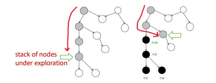
When DFS a graph, we will record two time stamp of each vertex:
- $d[u]$: Discover Time, when $u$ is first visited.
- $f[u]$: Finish Time, when we finish exploring all neighbors of $u$.
Of course, it's easy to see that $u.d < u.f$
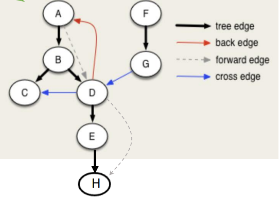
Then we can get $4$ different type of edges, for a $u \to v$:
- Tree Edge: When we first discover a new vertex $v$ from $u$.
- $u.d < v.d < v.f < u.f$
- Back Edge: An edge that points back to an ancestor in the DFS tree.
- $v.d < u.d < u.f < v.f$
- Forward Edge: An edge that goes from a node to its descendant in the DFS tree, but not a direct tree edge.
- $u.d < v.d < v.f < u.f$
- Cross Edge: An edge that goes between two different DFS branches (neither ancestor nor descendant).
- $v.d < v.f < u.d < u.f$
White Path Theorem
We colored the vertex in DFS:
- White: Not yet visited
- Gray: Currently being explored
- Black: Finished exploring
If, during a DFS, there is a path from a vertex $u$ to a vertex $v$ that only goes through white vertices, then $v$ will become a descendant of $u$ in the DFS tree.
We can use it to detect cycle in graph: When we see a back edge, or meet grey node, means we found a path from a node $u$ back to one of its ancestors $v$, and there is a cycle.
Topological Sort
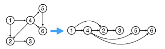
Topological Sort of a DAG $G=(V,E)$.
Theorem: $G$ is a DAG iff there is a linear ordering of all its $v \in V$ s.t., if $(u, v) \in E$, then $u < v$ in the above ordering. Or we say $(u,v)$ goes always from left to right.
Algorithm: Given DAG $G$.
- Run any DFS($G$), compute finishing time of nodes.
- Linear order: The nodes in decreasing order of finishing times.
Corollary: In a DAG, $(u, v) \in E \iff u.f > v.f$ for any DFS.
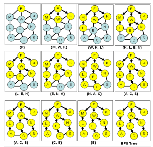
BFS
Breath-First Search (BFS) is searching neighbors around each node. And we usually use queue to implement.
Used very often in Shortest Path Algorithms.
int n, m;
vector <int> g[MAXN];
bool vis[MAXN];

void bfs(int st) {
    queue <int> q;
    q.push(st);
    vis[st] = true;
    while(!q.empty()) {
        int u = q.front(); q.pop();
        for(int x = 0; x < g[u].size(); x++) {
            int v = g[u][x];
            if(!vis[v]) {
                vis[v] = true;
                q.push(v);
            }
        }
    }
}
SCC
Strongly Connected Component (SCC): Maximal set of vertices $C \subseteq V$ such that for every pair of vertices $u, v \in C$, we have both $u \leadsto v$ and $v \leadsto u$.
$u \leadsto v$ means there is a path from $u$ to $v$.
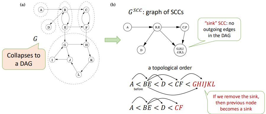
Kosaraju's Algorithm
Goal: Find all SCCs.
Key Observation: If you collapse each SCC into a single node, the resulting graph is a DAG. This DAG has a topological order.
If you start a DFS on a node located in a sink SCC (an SCC with no outgoing edges in the SCC DAG), the DFS will visit all nodes within that SCC and then stop, without leaking into other SCCs. You could then remove this SCC and repeat the process.
Idea: Reverse the direction of all edges in $G$ to create the transpose graph $G^T$.
int n, m;
vector<int> g[MAXN];      // original graph
vector<int> gr[MAXN];     // reversed graph
int vis[MAXN];
int d[MAXN], f[MAXN], cnt;
vector<int> order;        // store vertices by finish time
vector<int> component;    // store one SCC

void dfs1(int u) {
    vis[u] = 1;
    cnt++;
    d[u] = cnt;
    for (int v : g[u]) {
        if (!vis[v])
            dfs1(v);
    }
    cnt++;
    f[u] = cnt;
    order.push_back(u); // store vertex by finish time
    vis[u] = 2;
}

void dfs2(int u) {
    vis[u] = 1;
    component.push_back(u);
    for (int v : gr[u]) {
        if (!vis[v])
            dfs2(v);
    }
}

// Kosaraju main
void kosaraju() {
    cnt = 0;
    memset(vis, 0, sizeof(vis));
    for (int i = 1; i <= n; i++) {
        if (!vis[i])
            dfs1(i);
    }
    memset(vis, 0, sizeof(vis));
    reverse(order.begin(), order.end());
    cout << "Strongly Connected Components:\n";
    for (int u : order) {
        if (!vis[u]) {
            component.clear();
            dfs2(u);
            for (int x : component) cout << x << " ";
            cout << "\n";
        }
    }
}
And we can find all the SCCs using 2 DFS, with time complexity $O(n + m)$.
After Midterm (1 DAY BEFORE FINAL)
妈的,没时间了,得赶紧速通了
最短路(单源)
对于一个图 $G(V,E)$,其中两点 $u, v \in V$ 的最短路长度定义为 $\delta(u, v)$,且容易得到: $$ \delta(s, t) \leq \delta(s, u) + \delta(u, t) $$
Bellman-Ford
核心思想:对所有边执行 $n-1$ 轮松弛,复杂度 $O(nm)$
struct Edge {
    int u, v;
    LL w;
};

vector<Edge> edges;
vector<LL> dist;
int n, m, s;

bool bellman_ford() {
    dist.assign(n + 1, LLONG_MAX);
    dist[s] = 0;

    // n-1 次松弛
    for (int i = 1; i <= n - 1; i++) {
        bool updated = false;
        for (auto &e : edges) {
            if (dist[e.u] != LLONG_MAX &&
                dist[e.u] + e.w < dist[e.v]) {
                dist[e.v] = dist[e.u] + e.w;
                updated = true;
            }
        }
        if (!updated) break; // 提前结束
    }

    // 第 n 次检查负环
    for (auto &e : edges) {
        if (dist[e.u] != LLONG_MAX &&
            dist[e.u] + e.w < dist[e.v]) {
            return false; // 有负环
        }
    }
    return true; // 无负环
}
Dijkstra
核心思想:每一步都“贪心”地确定一个当前距离最小的点,并且一旦确定,就不会被更改。
算法维护两个集合:一个 $S$ 表示最短路已经被确定的点,还有一个 $V-S$ 表示还没被确定的点。每一步做三件事:
- 在 $V-S$ 中找到 $d$ 最小的点 $u$
- 把 $u$ 加入 $S$
- 用 $u$ 去松弛所有出边
那么,这个 $u$ 总是当前离 $s$ 最近的未确定点,不可能被绕路更短。
注意:没有负权的情况下
struct node {
	int v, dis;
};

struct pri {
	int ans, id;
	bool operator < (const pri &x) const{return x.ans < ans;}
};

priority_queue <pri> q;
vector <node> g[MAXN];
int n, m, d[MAXN], pre[MAXN];
bool vis[MAXN];

void Dijkstra(int st) {
	for(int x = 1; x <= n; x++) {
        d[x] = INF;
        pre[x] = -1;
        vis[x] = false;
    }
	d[st] = 0;
	q.push((pri){0, st});
	while(!q.empty()) {
		pri tmp = q.top();
		q.pop();
		int u = tmp.id;
		if(!vis[u]) {
			vis[u] = true;
			for(int y = 0; y < g[u].size(); y++) {
				int v = g[u][y].v;
				if(!vis[v] && d[u] + g[u][y].dis < d[v]) {
					d[v] = d[u] + g[u][y].dis;
                    pre[v] = u;
                    q.push((pri){d[v], v});
				}
			}
		}
	}
}

// 从ed回溯
void printPath(int ed) {
    vector <int> ans;
    for(int u = ed; u != -1; u = pre[u]) ans.push_back(u);
    reverse(ans.begin(), ans.end());
    for(int u : ans) cout << u << " ";
    cout << endl;
}
A*
可以立即为 Dijkstra 的升级版,对比:
- Dijkstra: priority = $g(v)$: past cost = cost to reach $v$
- A*: priority = $f(v)$ = $g(v) + h(v)$
其中,$h(v)$ 是一个启发式函数,在二维平面 A* 算法中,一般是用 $v$ 到终点的欧几里得距离。
struct node {
    int x, y;
    double val;
    bool operator < (const node &a) const {
        return val > a.val;
    }
} pre[MAXN][MAXN];

int dx[8] = {0, 1, 0, -1, 1, 1, -1, -1}, dy[8] = {1, 0, -1, 0, 1, -1, 1, -1};
string s[MAXN];
int g[MAXN][MAXN];
double f[MAXN][MAXN];
bool vis[MAXN][MAXN];
int n, m, ex, ey;
vector <node> ansPath;

double hfun(int ux, int uy) {
    return sqrt((double)((ux-ex)*(ux-ex)+(uy-ey)*(uy-ey)));
}

void buildPath() {
    int ux = ex, uy = ey;
    while(!(ux == -1 && uy == -1)) {
        ansPath.push_back((node){ux, uy, 0});
        int vx = pre[ux][uy].x, vy = pre[ux][uy].y;
        ux = vx, uy = vy;
    }
}

void AStar(int sx, int sy) {
    cout << "A*: " << sx << " " << sy << "-> " << ex << " " << ey << endl;
    for(int x = 0; x < n; x++) {
        for(int y = 0; y < m; y++) g[x][y] = INF;
    }
    g[sx][sy] = 0;
    f[sx][sy] = hfun(sx, sy);
    pre[sx][sy] = (node){-1, -1};

    priority_queue <node> q;
    q.push((node){sx, sy, f[sx][sy]});
    while(!q.empty()) {
        node tmp = q.top(); q.pop();
        int ux = tmp.x, uy = tmp.y, val = tmp.val;
        if(vis[ux][uy]) continue;
        vis[ux][uy] = true;
        if(ux == ex && uy == ey) {
            buildPath();
            return;
        }
        for(int o = 0; o < 8; o++) {
            int vx = ux + dx[o], vy = uy + dy[o];
            if(vx < 0 || vx >= n || vy < 0 || vy >= m) continue;
            if(s[vx][vy] == '*') continue;
            int tmpg = g[ux][uy] + 1;
            if(tmpg < g[vx][vy]) {
                pre[vx][vy] = (node){ux, uy, 0};
                g[vx][vy] = tmpg;
                f[vx][vy] = g[vx][vy] + hfun(vx, vy);
                q.push((node){vx, vy, f[vx][vy]});
            }
        }
    }
}
贪心
最小生成树
Kruskal算法:不停地添加下一个最短且不会生成环的边,用并查集维护。
struct edge {
	int u, v, w;
} e[MAXN];

int n, m;
int fa[MAXN];
vector <edge> MST;

bool cmp(edge x, edge y) {
	return x.w < y.w;
}

int find(int x) {
	return fa[x] == x ? x : fa[x] = find(fa[x]);
}

int Kruskal() {
	for(int x = 1; x <= n; x++) fa[x] = x;
	int ans = 0;
	sort(e+1, e+m+1, cmp);
	for(int x = 1; x <= m; x++) {
		int u = find(e[x].u), v = find(e[x].v);
		if(u == v) continue;
		fa[v] = u;
		ans += e[x].w;
		MST.push_back(e[x]);
	}
	return ans;
}
Prim 最小生成树:从任意一个点出发,每一步选择一条“连接已选点集和未选点集的最小边权”。
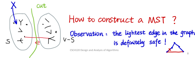
需要理解割定理(Cut Property):
对于一个图 $G(V,E)$来说,其割就是将图中所有顶点分成两个不重叠的集合 $S$ 和 $V-S$,割边就是连接这两个集合的边。
那么,在一个连通加权无向图中,对于任意一个割 $(S,V-S)$,如果某条割边 $e$ 的权重是所有割边里面最小的,那么这条边 $e$ 一定属于该图的某棵最小生成树。
证明可以用反证法,很简单。
Prim最小生成树的实现细节和 Dijkstra 非常像,都是维护一个小根堆,每次贪心地加边。
Huffman 编码
用于无损压缩储存字符串,让一个字符串里面出现频率高的字符编码短,频率低的字符编码长一些,传统方法是所有字符编码长度一样。
Huffman树:一棵 $01$ 前缀二叉树,左 $0$ 右 $1$。
给定一组符号 $c_1, c_2, \cdots, c_n$ 和每个符号出现的频率(权值)$w_i$,目标是构建一棵二叉树,每个符号对应一个叶子节点,使得带权路径长度($W$)最小
$$ \text{minimize } W = \sum_{i=1}^n w_i \cdot \text{depth}(c_i) $$
核心思想(贪心):每次合并当前权值最小的两个节点。
还是用小根堆来维护。
而且 Huffman 编码通过构建前缀二叉树,保证了没有任何一个字符的编码是另一个字符编码的前缀,这样在解码的时候也不会有歧义。
解码就很简单了,直接对应 Huffman 树从根往下走,走到叶子节点就将其输出,然后再回到根。
动态规划
之前写过两篇 blog 关于 DP 的,可以简单参考一下
动态规划就是把一个复杂的大问题,拆解成一个个重复的小问题,并把小问题的答案记录下来,最后得到大问题的答案。
最重要的是无后效性,即“未来与过去无关,只与现在有关”。一旦某个状态被确定,它是怎么到达这个状态的,无关紧要!后续的决策只依赖于当前状态。
如何设计一个 DP 方程:
- 定义状态(State):为了描述当前的局面,我需要知道哪些变量?状态必须包含所有“会限制未来决策”的信息。
- 定义选择(Choice):在当前状态下,我能进行什么操作?
- 明确 DP 数组的含义(Definition):用语言将 $dp[\dots]$ 的定义写下来,一定要具体。
- 写出状态转移方程(Transition):把选择变成数学公式,通常是
min,max或者sum。
$$ 现在的状态=择优 (之前的状态+本次选择的代价/收益) $$
Floyd 算法(多源最短路)
定义 $$ dp^{(k)}[i][j]=只允许使用 {1,2,\cdots,k} 作为中间点时,i \to j 的最短路 $$
状态转移方程 $$ dp^{(k)}[i][j] = \min\{dp^{(k-1)}[i][j], dp^{(k-1)}[i][k] + dp^{(k-1)}[k][j] \} $$
int n, m;
int d[MAXN][MAXN];
bool findN;

void Floyd() {
	findN = false;
	for(int k = 1; k <= n; k++)
		for(int i = 1; i <= n; i++)
			for(int j = 1; j <= n; j++)
				if(d[i][k] < INF && d[k][j] < INF)
					d[i][y] = min(d[i][j], d[i][k] + d[k][j]);
	for(int x = 1; x <= n; x++)
		if(d[x][x] < 0) findN = true; // 找到负环
}
区间 DP
核心思想:大区间的解=小区间的解+合并代价
标准套路:定义 $dp[i][j]$ 表示区间 $[i, j]$ 经过一系列操作之后得到的最优解。
状态转移方程:为了求 $dp[i][j]$,我们把区间 $[i, j]$ 从中间切一刀,分成 $[i, k]$ 和 $[k+1, j]$,枚举这个分割点 $k$,找到最优解。
$$ dp[i][j] = \min_{i \leq k < j}{ dp[i][k] + dp[k+1][j] } + \text{Cost}(i, j) $$
其中,$\text{Cost}(i, j)$ 是将两部分合并产生的代价。
遍历顺序:按照区间长度从小到大枚举。先算长度 $1$ 的区间,再算长度 $2$ 的区间,以此类推,最后能得到整个大区间的最优解。
最长公共子序列 LCS
给定两个字符串,找到它们的最长公共子序列(不要求连续)。
状态转移方程: $$ dp[i][j] = \begin{cases} dp[i-1][j-1] + 1 & \text{if } s1[i] = s2[j] \\ \max \{dp[i-1][j], dp[i][j-1] \} & \text{otherwise}\end{cases} $$ 其中 $dp[i][j]$ 表示 $s1$ 的前 $i$ 个字符和 $s2$ 的前 $j$ 个字符的 LCS 长度。
旅行商问题 TSP
定义状态 $dp[mask][i]$: $mask$ 是一个二进制转化成十进制的数,其 $n$ 位二进制表示已经访问过的城市集合;$i$ 表示当前停留在哪个城市(一定要在 $mask$ 里)。其值表示从起点出发,访问了 $mask$ 里所有城市,最后停在 $i$ 的最小总距离。
状态转移:假设我们在状态 $dp[mask][i]$,那么上一步我们在一个没访问 $i$ 之前的状态,停在某个 $j$。
之前的集合 $prev\_ mask$ 可以表示为 $mask \text{ xor } (1 << i)$,也就是把 $mask$ 里第 $i$ 位的 $1$ 去掉。
那么状态转移方程: $$ dp[mask][i] = \min_{j \in prev\_ mask} \{dp[prev\_ mask][j] + d[j][i] \} $$
void TSP() {
    cin >> n;
    for (int i = 0; i < n; i++)
        for (int j = 0; j < n; j++)
            cin >> w[i][j];
    int full = (1 << n);
    for (int mask = 0; mask < full; mask++)
        for (int i = 0; i < n; i++)
            dp[mask][i] = INF;
    dp[1 << 0][0] = 0;

    for (int mask = 0; mask < full; mask++) {
        if (!(mask & 1)) continue;
        for (int i = 0; i < n; i++) {
            if (!(mask & (1 << i))) continue;
            int prev = mask ^ (1 << i);
            if (prev == 0 && i != 0) continue;
            for (int j = 0; j < n; j++) {
                if (!(prev & (1 << j))) continue;
                dp[mask][i] = min( dp[mask][i], dp[prev][j] + w[j][i]);
            }
        }
    }

    int ans = INF, all = full - 1;
    for (int i = 1; i < n; i++) {
        ans = min(ans, dp[all][i] + w[i][0]);
    }
    cout << ans << "\n";
}
背包问题
01 背包:
有 $n$ 个物品,物品重量 $w_i$,价值 $v_i$,每个物品最多只能拿一个,背包大小 $S$。 $$ dp[i][j] = \max\{dp[i-1][j], dp[i-1][j-w[i]]+v[i] \} $$ 其中 $dp[i][j]$ 表示前 $i$ 个物品在容量 $j$ 下的最大价值。
void Knapsack01() {
    int S, n;
    cin >> S >> n;
    for(int x = 1; x <= n; x++) cin >> w[x] >> v[x];
    for(int j = 0; j <= S; j++) {
        for(int i = 1; i <= n; i++) {
            if(j-w[i] < 0) dp[i][j] = dp[i-1][j];
            else dp[i][j] = max(dp[i-1][j], dp[i-1][j-w[i]] + v[i]);
        }
    }
    cout << dp[n][S] << endl;
}
时间复杂度 $O(nS)$
完全背包:
同上,但可以重复拿 $$ dp[j] = \max \{dp[j-1], \max_i{dp[j-w[i]]+v[i] } \} $$ 其中 $dp[j]$ 表示容量 $j$ 下的最大价值。
void KnapsackComplete() {
    int S, n;
    cin >> S >> n;
    for(int x = 1; x <= n; x++) cin >> w[x] >> v[x];
    for(int j = 0; j <= S; j++) {
        for(int i = 1; i <= n; i++) {
            if(j-w[i] >= 0)
                dp[j] = max(dp[j], dp[j-w[i]] + v[i]);
        }
    }
    cout << dp[S] << endl;
}
时间复杂度 $O(nS)$
平衡划分问题
给定一个包含 $n$ 个正整数的集合,如何将其划分为两个子集,使得这两个子集的元素和相差最小。
$$ \min_{S_1, S_2} d = \left| \sum_{i \in S_1} k_i - \sum_{j \in S_2} k_j \right| $$
核心解法:将其转化为 01 背包问题。先算出总和 $\text{Sum}$,找到一个子集使其和尽可能接近 $\frac{\text{Sum}}{2}$,然后就是一个容量为 $\frac{\text{Sum}}{2}$ 的 01 背包问题了,每个物品的价值和重量都是它本身,EZ。
网络流
想象一个由管道组成的网络:
- 源点(Source, $S$):自来水厂,有无限的水流出
- 汇点(Sink, $T$):大海,可以接收无限的水
- 容量(Capacity, $c$):每根管道 $(u,v)$ 单位时间最多能流过的水量
- 流量(Flow, $f$):实际流过的水量
还有以下规则:
- 流量限制:$f(u,v) \leq c(u,v)$(水管不能撑爆)
- 流量守恒:对于除了 $S$ 和 $T$ 以外的任意节点,流入量=流出量
那么问题:在不撑爆任何管道的前提下,从源点 $S$ 最多能推多少水到汇点 $T$?
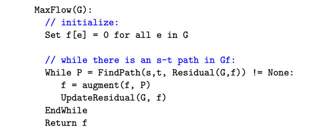
Ford-Fulkerson 方法
核心思想:只要还能找到一条路去推流,就往死里推;推不动了,现在的流量就是最大流。
这条“能推流的路”叫做增广路(Augmenting Path)
反向边:如果随便找了一条路推流,可能会堵死另一条更优的路线,那么可以加一个反向边,每当我们在边 $(u,v)$ 上推了 $k$ 的流量:
- 正向边的 $c(u,v)$ 减少 $k$
- 反向边的 $c(v,u)$ 增加 $k$
在残量网络(Residual Graph)中走反向边,相当于“撤销”之前的操作!
Edmonds-Karp 算法
用 BFS 在参量网络图里寻找增广路,确保每次找的都是边数最少的路。
这里的增广路是包括反向边的,但要满足硬性条件:剩余容量(Capacity)$>0$
BFS 总能找到经过边数最少的那条增广路(最短路性质),可以保证效率是 $O(nm)$,然后再乘上更新一次推流的复杂度 $O(m)$,使得算法总复杂度 $O(nm^2)$
LL BFS()
{
	memset(last, -1, sizeof(last));
	queue <LL> q;
	q.push(s);
	flow[s] = INF;
	while(!q.empty())
	{
		int u = q.front(); q.pop();
		if(u == t) break;
		for(LL x = head[u]; x > 0; x = edge[x].next)
		{
			LL v = edge[x].to, w = edge[x].w;
			if(w > 0 && last[v] == -1)
			{
				last[v] = x;
				flow[v] = min(flow[u], w);
				q.push(v);
			}
		}
	}
	return last[t] != -1;
}

LL EK()
{
	LL ans = 0;
	while(BFS())
	{
		ans += flow[t];
		for(LL x = t; x != s; x = edge[last[x] ^ 1].to)
		{
			edge[last[x]].w -= flow[t];
			edge[last[x]^1].w += flow[t];
		}
	}
	return ans;
}
代码是古早时期用链式前向星随便写的,凑合着看吧(
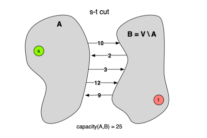
最大流最小割定理
Max-Flow Min-Cut Theorem
割的定义是顶点的集合,在网络流中特指 $s-t$ 割,即我们将顶点集合 $V$ 划分成 $S$ 和 $TY$,使得:
- 源点 $s \in S$
- 汇点 $t \in T$
- $S \cup T = V$ 且 $S \cap T \empty$
割的容量,记为 $C(S,T)$,是指所有从 $S$ 指向 $T$ 的边的容量之和。 $$ C(S,T) = \sum_{u \in S, v \in T} c(u,v) $$
复杂度
以下内容由 Gemini 生成
这四个概念(P, NP, NP-Hard, NP-Complete)是理论计算机科学的基石,但名字起得非常容易让人误解。
最常见的误区是:“NP 就是 Not Polynomial(非多项式),就是难解的问题。” —— 这是大错特错的!
我们要用验算和归约这两个视角来彻底搞懂它们。
1. P (Polynomial Time) —— “能做出来的”
定义:能在多项式时间 $O(n^k)$ 内解决的问题。 直观:计算机能快速搞定的问题。
- 例子:
- 给你一个数组,把它排个序。(归并排序 $O(n \log n)$)
- 给你个地图,找两点间最短路。(Dijkstra $O(E \log V)$)
- 判断一个数是不是偶数。($O(1)$)
2. NP (Nondeterministic Polynomial Time) —— “能检查答案的”
名字误区:NP 不代表“非多项式(Non-Polynomial)”,它代表“非确定性多项式(Non-deterministic Polynomial)”。这个名字来源于非确定性图灵机,比较抽象,你可以直接忽略它。
真正的定义(验证视角): 如果在多项式时间内,给定一个“解(Certificate/Witness)”,你能验证这个解是不是对的,那这个问题就在 NP 里。
直观:虽然我不会做,但如果你蒙了一个答案给我,我能很快告诉你蒙得对不对。
- 例子(数独):
- 让你解一个 $100 \times 100$ 的空数独,这极难(可能是指数级时间)。
- 但是,如果我直接塞给你一张填满了数字的纸,问你“这是不是解?”,你只需要扫描一遍行、列、宫,几秒钟就能告诉我 Yes 或 No。
- 所以,数独属于 NP。
P 和 NP 的关系:
- $P \subseteq NP$。
- 为什么?因为如果你能快速解出问题,那你当然也能快速验证答案(直接解一遍对比一下就行了)。
- 千古之谜:$P = NP$ 吗?(即:所有能被快速验证的问题,都能被快速解决吗?目前绝大多数科学家认为 $P \neq NP$)。
3. NP-Hard —— “大Boss”
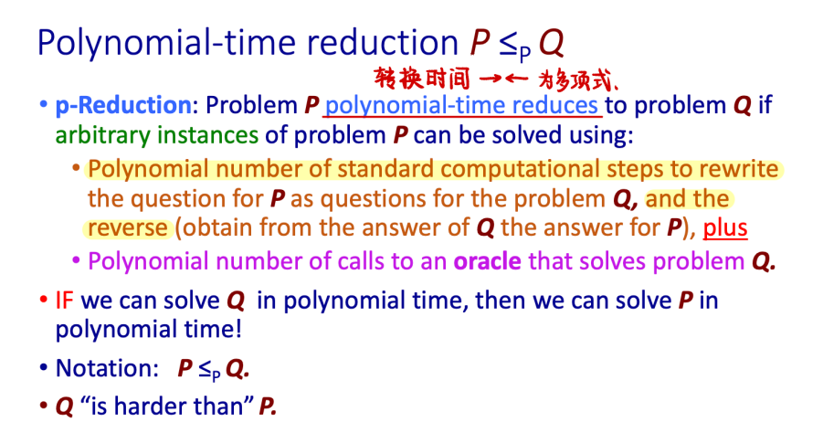
定义:如果所有的 NP 问题都能在多项式时间内归约到问题 X,那么 X 就是 NP-Hard。
通俗翻译: “我是个狠角色。如果谁能把我也在多项式时间内解决了,那么世界上所有的 NP 问题(比如数独、TSP、图着色)就全都解决了。”
特点:
- 它不一定在 NP 里:NP-Hard 问题甚至可能连“验证答案”都很难。
- 它代表了“难度下限”:它至少和 NP 中最难的问题一样难。
- 例子:
- 停机问题:给定一段代码,判断它会不会死循环。这是不可解的,它比所有 NP 问题都难,所以它是 NP-Hard,但它不是 NP(因为连验算都做不到)。
4. NP-Complete (NPC) —— “NP 里的扛把子”
定义:一个问题如果满足两个条件,它就是 NPC:
- 它属于 NP(能被快速验证)。
- 它属于 NP-Hard(所有 NP 问题都能归约给它)。
直观: 它是 NP 集合里最难、最核心的那一小撮问题。它们处于 P/NP 图解的交界处。 NPC 问题的神奇之处在于它们的等价性:只要你解决了其中任何一个 NPC 问题(找到多项式算法),你就解决了所有的 NP 问题(即证明了 P=NP)。
- 经典 NPC 例子:
- SAT (布尔可满足性问题):第一个被证明是 NPC 的问题(祖师爷)。
- TSP (旅行商问题-判定版):给一个长度 $L$,问有没有一条路径长度小于 $L$?
- 最大团问题:图里有没有 $K$ 个点两两相连?
- 背包问题。
5. 总结与辨析(一张表看懂)
| 类别 | 核心能力 | 通俗理解 | 典型例子 |
|---|---|---|---|
| P | 能解决 | 简单题,电脑跑得飞快 | 排序、最短路、最小生成树 |
| NP | 能验证 | 只有上帝或欧皇能猜中答案,但我能检查对不对 | 数独、因数分解、以及所有 P 问题 |
| NPC | 能验证 + 最难 | NP 里的万恶之源。解出一个就能解出所有。 | SAT、TSP(判定)、图着色 |
| NP-Hard | 未必能验证 + 极难 | 难度无上限,包含了 NPC 和比 NPC 更难的问题 | 停机问题、TSP(优化版)、围棋必胜策略 |
6. 一个常考的细节:优化 vs 判定
通常我们在算法书上讨论 P/NP 时,讨论的都是判定问题(Decision Problem),即答案只有 Yes/No 的问题。
- TSP 优化版:“求最短路径是多少?” $\to$ 这是 NP-Hard。
- TSP 判定版:“是否存在一条路径长度 $< 100$?” $\to$ 这是 NP-Complete。
为什么? 因为“优化版”不好验证。如果我给你一条路,说“这是最短的”,你怎么验证它是最短的?你很难在多项式时间内验证没有更短的路。 但“判定版”很好验证。我给你一条小于 100 的路,你算一下长度,确实小于 100,验证通过。
总结
- P:做起来容易。
- NP:检查起来容易。
- NPC:NP 里最难的,如果攻克它,世界将发生巨变(密码学崩溃)。
- NP-Hard:只要能把所有 NP 问题转化成它,它就是 NP-Hard。
下次有人问你,你可以装作很深沉地说:“P 是解的集合,NP 是验证的集合,NPC 是这帮验证问题里的终极代理人。”