DDA3005: Numerical Methods

L1 Introduction to Numerical Methods

Numerical Methods

Main Goal: Design and analysis of algorithms for solving mathematical problems arising in science and engineering numerically.

Features:

• Deal with continuous quantities(time, distance, velocity, tempreature, density and pressure) typically measured by real numbers.
• Consider effects of approximations.
• Use scientific computing and computer simulations to understand natural phenomena.
• Simulations and algorithms allow to build accessible and cheap virtual prototypes of engineering problems: "build-and-test". 虚拟样机

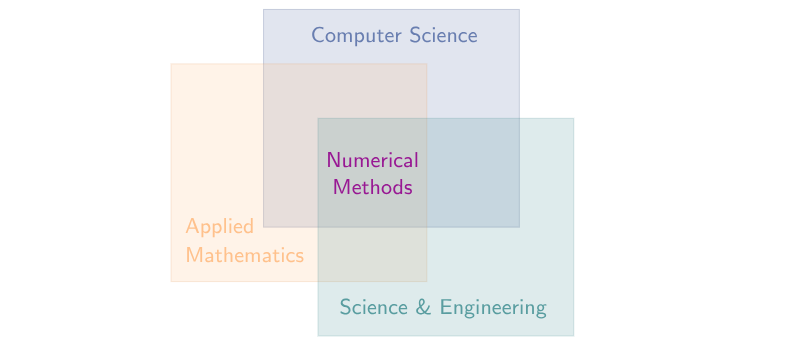
General Mathematical Problems

Consider a function:

$$ y=f(x) $$

And we have typical problems:

1. Evaluate a function: given x, output y.
2. Solve an equation: given y, find x.
3. Optimize: find x that yields optimal y.

When thinking about the problems, we should consider:

• Discrete or Continuous(Concrete)
• Linear or Nonlinear
• Finite or Inifinite Dimensional
• Purely Algebraic or Involve derivatives or Integrals

And we have strategies like:

• Differential $\to$ Algebraic
• Nonlinear $\to$ Linear
• Complicated $\to$ Simple

The obtained solution might only approximate the true solution of the original problem.

Example 1: Image Deblurring

Consider a blurry image, knowing the type of blurring can we reconstruct the original image?

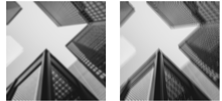
We assume that blurring is a linear operation:

$$ Ax = b $$

where $b$ is the given blurry image (in vector form), $A$ represents the blurring operation and $x$ is the original image that we want to find and reconstruct.

We can obtain $x$ by simple matrix inversion:

$$ x = A^{-1} b $$

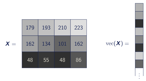
A grayscale image with $m \times n$ pixels is usually represented as a matrix $X \in \mathbb{R}^{m \times n}$. And we can tranform it to vector $x = \text{vec}(X) \in \mathbb{R}^{mn}$ firstly.

The blurring operation is modeled via a blurring kernal $W \in \mathbb{R}^{s \times t}$ (point spread function) and satisfies $\sum_{i,j} w_{ij}=1$, for example:

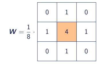
And we can apply the blurring kernal over each pixel $x_{ij}$, like performing a local average.

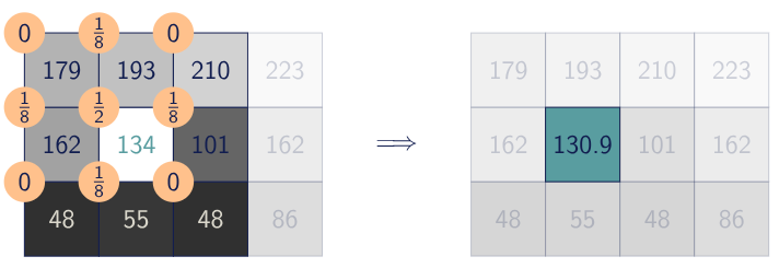
So, to obtain the original image from the blurred image $b = \text{vec}(B)$, we can solve the linear system of equations:

$$ Ax = A \cdot \text{vec}(X) = \text{vec}(B) = b $$

Questions and Challenges:

• How can we solve linear systems $Ax=b$ on a computer?
• Can we describe / explain the observed phenomenon mathematically?
• The tested image has $1024 \times 1024$ pixels in total, hence $A$ is a matrix of $1048576 \times 1048576$, how can we deal with it?

Example 2: Large-Scale Optimizaiton

Many machine learning problems can be expressed in the form:

$$ \min_{w \in \mathbb{R}^n} f(w) := \frac1N \sum_{i=1}^N f_i(w) $$

where each $f_i: \mathbb{R}^n \to \mathbb{R}$ is smoothe and $N \in \mathbb{N}$ is given.

Each $f_i$ satisfis $f_i(w) = \ell(w, \xi_i)$ where $\ell: \mathbb{R}^n \times \mathbb{R}^m \to \mathbb{R}$ is the common loss function.

Support Vector Machines (SVM).

L2 Floating-Point Numbers and Arithemtic

Floating-Point Numbers

Consider the memory architecture in computers:

Observation:

• There are only finitely many memory cells.
• Only finitely many numbers are representable on a computer.

The floating-point number system is characterized by four integers:

• $\beta$: base or radix
• $p$: precision
• $[L,U]$: exponent range

A real lnumber $x$ is represented as:

$$ x = \pm \left[ d_0 + \frac{d_1}{\beta} + \frac{d_2}{\beta^2} + \cdots + \frac{d_{p-1}}{\beta^{p-1}} \right]\beta^E $$

where $0 \le d_i \le \beta-1, i = 0, \cdots, p-1$ and $L \le E \le U$.

And we usually have:

• $E$: exponent 指数
• $d_0.d_1 d_2 \cdots d_{p-1}$: mantissa 尾数
• $d_1 d_2 \cdots d_{p-1}$: fraction 小数部分

e.g. Let us set $\beta=10$ and $p=7$, we can write:

$$ \begin{aligned} 0.1 &= + 0.100000 \cdot 10^0\\ 31.41592 &= + 3.141592 \cdot 10^1 \end{aligned} $$

Normalization: The floating-point system is said to be normalized if the leading digit $d_0$ is always nonzero unless the represented number is zero. And the mantissa $m$ of a nonzero floating-point number always satisfies $1 \le m < \beta$

Properties:

• The floating-point number system is finite and discrete.
• Total number of normalized floating-point numbers in a system is: $$ 2(\beta-1)\beta^{p-1}(U-L+1)+1 $$
• Smallest positive normalized number: $$ \text{UFL} = \text{underflow level} = \beta^L $$
• Largest floating-point number: $$ \text{OFL} = \text{overflow level} = \beta^{U+1}(1-\beta^{-p}) $$

e.g. Floating-point system: Let us consider the system $\beta=2$, $p=3$, $L=-1$ and $U=1$, this system contains:

$$ 2 \cdot (2-1) \cdot 2^2 \cdot (2+1) + 1 = 25 $$

numbers in total and we hvae:

$$ \text{OFL} = (1.11)_{2} \cdot 2^1 = (1+\frac12+\frac14) \cdot 2 = (3.5)_{10} $$

$$ \text{UFL} = (1.00)_2 \cdot 2^{-1} = (1+0+0) \cdot \frac12 = (0.5)_{10} $$

All normalized floating-point systems look discrete and unequally spaced.

Rounding Rules:

If the real number $x$ is not representable, then it is approximated by a "nearby" floating-point number $\text{fl}(x)$.

Two commonly used rouding rules:

• Chop: truncatehte base-$\beta$ expansion of $x$ after the $(p-1)$st digit (round toward zero).
• Round to nearest: 四舍五入

Rounding to nearest is the most accurate and is the default rounding rule in IEEE systems.

Matchine Precision

The accuracy of a floating-point system is characterized by the unit roundoff(machine precision or machine epsilon), denoted by $\varepsilon_{\text{mach}}$:

• With rounding by chopping: $\varepsilon_{\text{mach}} = \beta^{1-p}$
• With rounding to nearest: $\varepsilon_{\text{mach}} = \frac12 \beta^{1-p}$

Alternatively, $\varepsilon_{\text{mach}}$ is defined as the smallest number $\varepsilon$ such that $\text{fl}(1+\varepsilon) > 1$.

Proposition: Rounding

For every $x \in \mathbb{R}$ in the range of the floating-point system, we have:

$$ |\text{fl}(x)-x| \le \varepsilon_{\text{mach}}|x| $$

or we can write in a more common way:

$$ \frac{|\text{fl}(x)-x|}{|x|} \le \varepsilon_{\text{mach}} $$

For IEEE floating-point systems:

• $\varepsilon_{\text{mach}} = 2^{-24} \approx 10^{-7}$ in single precision.
• $\varepsilon_{\text{mach}} = 2^{-53} \approx 10^{-16}$ in double precision.
• $\varepsilon_{\text{mach}} = 2^{-113} \approx 10^{-36}$ in quadruple precision.

Subnormals and Gradual Underflow

?

Exceptional Values

IEEE floating-point standards:

• Inf: "infinity", results from dividing a finite number by zero ($1/0$)
• NaN: "not a number", results from undefined or interminate operations such as $0/0, 0\cdot \text{Inf}$ or $\text{Inf}/\text{Inf}$.

L3 Floating-Point Arithmetic and Error Analysis

Floating-Point Arithmetic and Cancellation

Floating-Point Arithmetic:

• Addtion or Subtraction ($\oplus, \ominus$)
• Multiplication ($\odot$)
• Division ($\oslash$)

Results of these floating-point operations may diffier from results of the corresponding real arithmetic operation.

e.g. Let us set $\beta=10$ and $p=6$, and $x=1.92403 \cdot 10^2$ and $y=6.35782 \cdot 10^{-1}$ be given. We can get $$ x \oplus y = 1.93039 \cdot 10^2 $$ (use rounding to nearest)

Comments: The real result may fail to be representable because its exponent is byond the available range. Overflow is a serious problem as there is no good approximation to arbitrarily large numbers in floating-point systems.

e.g. Evaluating a Divergent Series:

$$ \sum_{k=1}^\infin \frac1k $$

is divergent, yet has finite value in floating-point arithmetic

Possible Explanations:

• The partial sum eventually overflows.
• $\frac1k$ eventually underflows.
• Partial sum ceases to change on $\frac1k$ becomes negligible relative to the partial sum $$ \frac1k < \varepsilon_{\text{mach}} \cdot \sum_{i=1}^{k-1} \frac1i $$

IEEE-Standard 754: For any operation $* \in {+,-,\cdot,/ }$ and any pair of machine numbers, we have

$$ x \circledast y = \text{fl}(x * y) $$

which means $x \circledast y = (1 + \varepsilon) \cdot (x*y)$ for sum $|\varepsilon| \le \varepsilon_{\text{mach}}$

Floating-point addition and multiplication are commutative but not associative.

e.g. If $\varepsilon$ is a positive floating-point number that is slightly smaller than $\varepsilon_{\text{mach}}$ then $(1 \oplus \varepsilon) \oplus \varepsilon = 1$ but $1 \oplus (\varepsilon \oplus \varepsilon) > 1$

Cancellation

Consider $\ominus$: If the two $p$-digit numbers having same sign and similar magnitudes yields results with fewer than $p$ digits, so it is usually exactly representable. The leading digits of the two numbers cancel (i.e. their difference is zero).

e.g. $$ 1.92403 \cdot 10^2 \ominus 1.92275 \cdot 10^2 = 1.28000 \cdot 10^{-1} $$

which is correct and exactly representable, but has only $3$ significant digits.

BUT, despite the exactness, cancellation often implies serious loss of information!

e.g. If $\varepsilon$ is a positive floating-point number that is slightly smaller than $\varepsilon_{\text{mach}}$ then

$$ (1 \oplus \varepsilon) \ominus (1 \ominus \varepsilon) = 1 \ominus 1 = 0 $$

The true result of the computation $2 \varepsilon$ has been completely lost!

e.g. Evaluating alternating series such as

$$ e^x = 1 + x + \frac{x^2}{2!} + \frac{x^3}{3!} + \cdots $$

for $x<0$ can give a disastrous result due to catastrophic cancellation.

e.g. Quadratic Formula: The two solutions of the quadratic equation $ax^2 + bx + c = 0$ are given by

$$ x_{1/2} = \frac{-b \pm \sqrt{b^2-4ac}}{2a} $$

A naive use of this formula can suffer from overflow, underflow or severe cancellation.

But the cancellation between $-b$ and the square root can be avoided by computing

$$ x_{1/2} = \frac{-b \pm \sqrt{b^2-4ac}}{2a} \cdot \frac{-b \pm \sqrt{b^2-4ac}}{-b \pm \sqrt{b^2-4ac}} = \frac{2c}{-b \mp \sqrt{b^2-4ac}} $$

Cancellation inside the square root cannot be easily avoided without using higher precision.

e.g. Standard Deviation: The mean and standard deviation of sequence $\{x_i\}_{i=1}^n$ are given by: $$ \bar{x} = \frac1n \sum_{i=1}^n x_i $$

$$ \sigma^2 = \frac1{n-1} \sum_{i=1}^n (x_i - \bar{x})^2. $$

The mathematically equivalent formula

$$ \sigma^2 = \frac1{n-1}\left( \sum_{i=1}^n x_i^2 - n \bar{x}^2 \right) $$

avoids making two passes through the data.

L4 Errors and Conditioning

Approximations and Errors

Absolute Error and Relative Error

Absolute Error: $\text{approximate value} - \text{true value}$

Relative Error: $\frac{\text{absolute value}}{\text{true value}}$

$\text{approx. value} = (\text{true value} \cdot (1 + \text{rel. error}))$

The true value is usually unknown, so we estimate or bound the error rather than compute it exactly.

Data Erorr and Computational Error

Typical problem: evaluate a function $f: \mathbb{R} \to \mathbb{R}$ for a given argument:

• $x$ = true value of input.
• $f(x)$ = corresponding output value for true function.
• $\hat{x}$ = approximate input actually used.
• $\hat{f}$ = approximate function actually used.

Total Error:

$$ \begin{aligned} \hat{f}(\hat{x}) - f(x) =& ( \hat{f}(\hat{x}) - f(\hat{x}) ) &&+ &&( f(\hat{x}) - f(x) ) \\ &\text{computational error} &&+ &&\text{propagated data error} \end{aligned} $$

Truncation Error and Rounding Error

Truncation Error: difference between true result and result produced by given algorithm by using exact arithmetic

Rounding Error: Difference between result produced by given algorithm using exact arithmetic and result produced by same algorithm using limited precision arithmetic.

Computational error is sum of truncation error and rounding error, where one of these usually dominates.

e.g. Finite Difference Approximation

Error in finite difference approximation

$$ f'(x) \approx \frac{f(x+h)-f(x)}h $$

exhibits trade-off between rounding error and truncation error.

• Truncation error is bounded by $\frac{Mh}2$ where $M$ bounds $|f''(t)|$ for $t$ near $x$.
• Rounding error is bounded by $\frac{2\varepsilon}h$ where the error in function values is assumed to be bounded by $\varepsilon$.
• Total error minimized when $h \approx 2 \sqrt{\frac{\varepsilon}M}$
• Error increases for smaller $h$ because of rounding error and increases for larger $h$ because of truncation error.

Forward and Backward Error

Suppose we want to compute $y=f(x)$ where $f: \mathbb{R} \to \mathbb{R}$, but we can only obtain an approximate value $\hat{y}$.

Forward Error: Difference between computed result $\hat{y}$ and the true output $y$:

$$ \Delta y = \hat{y} - y $$

Backward Error: Difference between actual input $x$ and input $\hat{x}$ for which computed result $\hat{y}$ is exactly correct:

$$ \Delta = \hat{x}-x $$

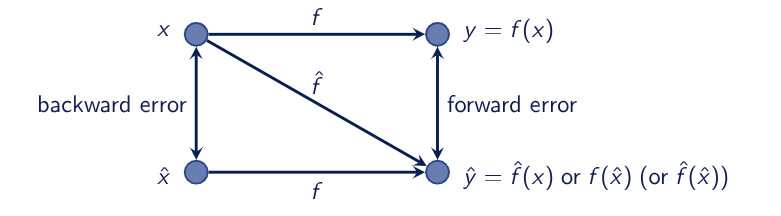
e.g. Approximating the cosine function $f(x) = \cos(x)$ by truncating its Taylor series after two terms gives

$$ \hat{y} = \hat{f}(x) = 1 - \frac{x^2}2 $$

• Forward error is giving by $$ \Delta y = \hat{y}-y = \hat{f}(x) - f(x) = 1 - \frac{x^2}2 - \cos(x). $$

• For $x=1$, this yields: $$ y = f(1) = \cos(1) \approx 0.5403 \\ \hat{y} = \hat{f}(1) = 1-\frac{1^2}2 = 0.5 \\ \hat{x} = \arccos(\hat{y}) = \arccos{0.5} \approx 1.0472 $$

• Forward error: $\Delta y = \hat{y}-y \approx 0.5 - 0.5403 = -0.0403$

• Backward error: $\Delta x = \hat{x}-x \approx 1.0472 - 1 = 0.0472$

L5 Conditioning, Stability and Accuracy

Repetition and Conditioning

Condition Number:

$$ \text{cond} = \frac{|\text{relative change in solution}|}{|\text{relative change in input data}|} = \frac{|(f(\hat{x}) - f(x))/f(x)|}{|(\hat{x} - x)/x|} = \frac{|\Delta y/y|}{|\Delta x/x|} $$

The problem is sensitive or ill-conditioned if $\text{cond} \gg 1$

The condition number is an amplificaiton factor relating the forward error to the relative backward error:

$$ |\text{relative forward error}| = \text{cond} \cdot |\text{relative backward error}| $$

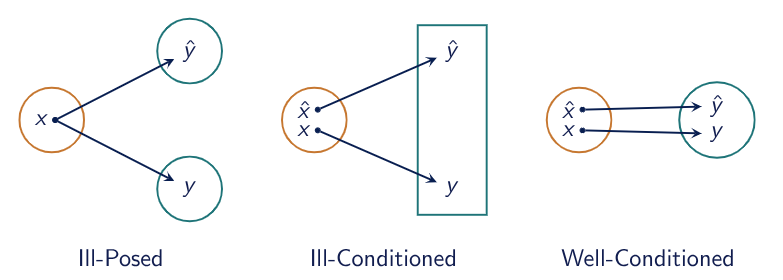
e.g. Consider a funciton:

$$ y = f(x) = x^2 $$

if a small change $\Delta x$ happens to $x$, we have

$$ \Delta y \approx f'(x) \Delta x = 2x \Delta x $$

So

$$ \text{cond} = \frac{|\Delta y/y|}{|\Delta x/x|} = 2 $$

It means that the error of output will be approximatly be $2$ times than $x$, such as if $x$ has error of $1%$, then $y=x^2$ will approximately have error of $2%$.

Mathematical Definition: The (relative) condition number of a problem $f: \mathbb{R} \to \mathbb{R}$ at a point $x$ can also be defined more rigorously as

$$ \text{cond}(x) = \kappa(x) := \lim_{\delta \to 0} \sup_{|\Delta x| \le \delta} \frac{|f(x+\Delta x) - f(x)|}{|f(x)|} \Bigg / \frac{|\Delta x|}{|x|} $$

If $f$ is differential at $x$, then this exactly gives $\text{cond}(x) = \frac{|x f'(x)|}{|f(x)|}$

Stability

An algorithm $\hat{f}$ for a problem $f$ is called stable if the produced result is relatively insensitive to perturbations during computation.

Mathematical Definition: An algorithm $\hat{f}: \mathbb{R}^n \to \mathbb{R}^m$ for a problem $f:\mathbb{R} \to \mathbb{R}^m$ is called stable if for all $x \in \mathbb{R}^n$, we have

$$ \frac{|\hat{f}(x) - f(\hat{x})|}{|f(x)|} = \mathcal{O}(\varepsilon_{\text{mach}}) \quad \text{for some } \hat{x} \text{ with } \frac{|\hat{x} - x|}{|x|} = \mathcal{O}(\varepsilon_{\text{mach}}). $$

Landau Notation: big-$\mathcal{O}$ and small-$\mathcal{o}$

Learned in CSC4120, skipped.

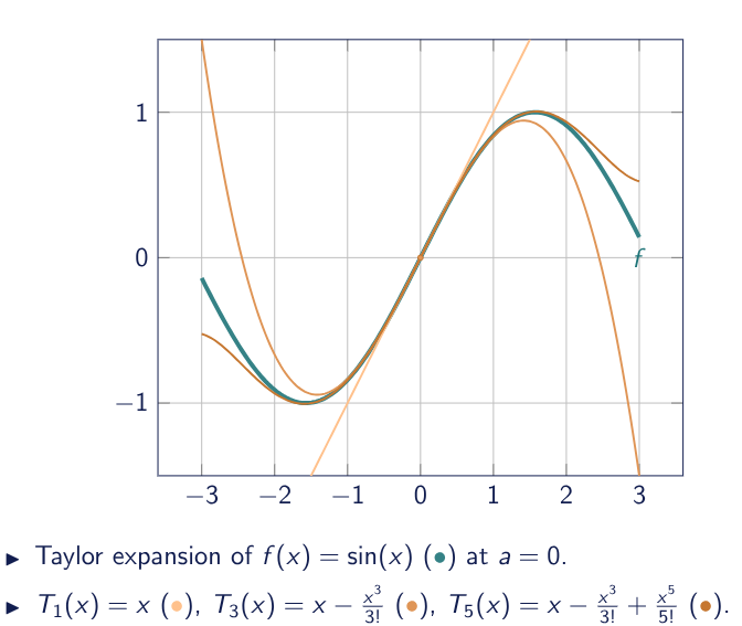
Taylor Expansion (review): Let $f: \mathbb{R} \to \mathbb{R}$ be $k$-times diff. at $a \in \mathbb{R}$, we have

$$ f(x) = \sum_{i=0}^k \frac{f^{(i)}(a)}{i!} (x-a)^i + R_k(x) $$

where $R_k(x) = \mathcal{o}(|x-a|^k)$ for $x \to a$ and $f^{(i)}(a)$ denotes the $i$-th derivative of $f$ and $a$.

Taylor's theorem allows to approximate a function by a polynomial expansion close to the reference point $a$.

e.g. Illustration of Taylor Expansion

Accuracy of Algorithms

Not finished.