Stochastic Processes
L0 Examples of Stochastic Processes
Example 1: Discrete Steps in Time
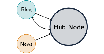
Imagine browsing the internet purely at random and navigating across an interconncted network of states (webpages).
The Fundamental Principle: Given where the system is right now, where it goes next is completely independent of how it got there.
Two Real-Wordl Dilemmas:
- The Dead End: A webpage that has not outgoing links.
- The Spider Trap: Two pages only link back and forth to each other.
Solution: Random Teleportaion
- Most of time (~85%): Follow an actual hyperlink on the page.
- Occasionally (~15%): Get bored, type a brand-new random URL.
After we clicked for a million times, we get the Google PageRank Intuition: The importance of a page is how long-run time spent on it. That is, more important the webpage is, the more frequent it will be clicked to.
Example 2: Events Across Continuous Time
Real-world events do not wait for discrete "clicks", they unfold in continuous time.
A stream of independent, unpredictable events with a steady average pace is a Poisson Process.
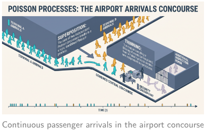
Consider Corridor A and Corridor B, passengers arrive at steady pace $\lambda_1$ and $\lambda_2$ for each corridor.
The Superposition Property: When independent Poisson streams merge, the combined stream is still a textbook Poisson process. And the combined rate simply adds up: $\lambda_{\text{total}} = \lambda_1 + \lambda_2$
Part I Review of Probability Tools
Mostly STA2001 contents.
The Inclusion-Exclusion Principle (De Moivre's Formula):
$$ \begin{aligned} P(A_1 \cup A_2 \cup \cdots \cup A_n) = & \sum_{A_i} P(A_i) \\ & - \sum_{A_i,A_j} P(A_i A_j) \\ & + \sum_{A_i,A_j,A_k} P(A_i A_j A_k) \\ & - \cdots \\ & + (-1)^{n-1} P(A_1 A_2 \cdots A_n) \end{aligned} $$
Numbers of terms in each sum: $\binom{n}{k}$
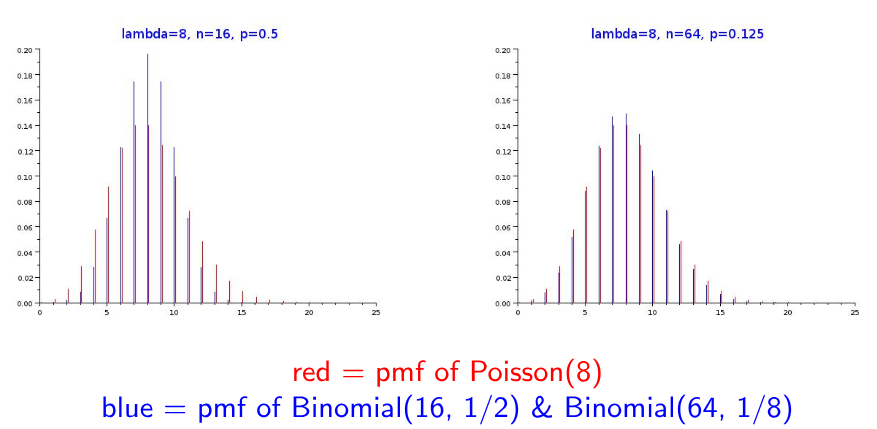
Poisson r.v. as limit of Binomial r.v.'s
Suppose that $X_n$ is a binomial r.v. with parameters $(n, p_n)$, and let $\lambda_n = n p_n \to \lambda$ when $n \to \infin$.
Then for any fixed $i$, we have
$$ P\{X_n=i\} = \lim_{n \to \infin} \frac{n!}{i!(n-i)!} p_n^i(1-p_n)^{n-i} \rightarrow e^{-\lambda}\frac{\lambda^i}{i!} $$
What does mean a density value $f(x)$?
Consider a pdf
$$ f(x) = \begin{cases} \frac{1}{x^2} & x \ge 1, \\ 0 & x < 1 \end{cases} $$
Then the meaning of $f(2) = \frac14$ will be: For small $\epsilon$, $P(2-\epsilon \le X \le 2+\epsilon) \approx \frac14 \cdot 2 \epsilon$
Or in formal we have:
Since $$ f(x) = F'(x) = \lim_{h\to 0} \frac{F(x+h)-f(x)}{h} $$
we have for small $h$, $$ P\{x < X \le x+h\} = F(x+h) - F(x) \approx h \cdot f(x) $$
Expectation of R.V.
For discrete r.v. $X$ with pmf $P(x)$, we have definition:
$$ E[X] = \sum_x x P(X=x) $$
Now, consider $N$ as a r.v. with natural numbers $1,2,3,\cdots$, then
$$ \begin{aligned} E[N] &=&& 1\cdot P(N=1) + 2\cdot P(N=2) + 3\cdot P(N=3) \\ &=&& P(N=1) + \\ &&&[P(N=2)+P(N=2)] + \\ &&&[P(N=3) + P(N=3) + P(N=3)]+\\ &&& \cdots\\ &=&& [P(N=1)+P(N=2)+P(N=3)+\cdots] + \\ &&& [P(N=2)+P(N=3)+P(N=4)+\cdots] + \\ &&& \cdots \\ &=&& P(N\ge 1) + P(N \ge 2) + P(N \ge 3) + \cdots \\ &=&& \sum_{n=0}^\infin P(N > n) \end{aligned} $$
We call it the formula of integer random variables.
e.g. There are $m$ kinds of cards, the probability of choosing the $i$ th card is $p_i$, we want to know the expectation $E[N]$ of getting all kinds of cards.
Consider $A_i = \{\text{didn't get }i\text{ th card in the previous } n \text{ times}\}$, then we have:
$$ \{N > n\} = A_1 \cup A_2 \cup \cdots \cup A_m $$
Use the Inclusion-Exclusion Principle:
$$ \begin{aligned} P(N>n) &= \sum_i P(A_i) - \sum_{i<j} P(A_i \cap A_j) + \sum_{i<j<k}P(A_i \cap A_j \cap A_k) - \cdots \\ &=\sum_i(1-p_i)^n - \sum_{i<j}(1-p_i-p_j)^n + \sum_{i<j<k}(1-p_i-p_j-p_k)^n - \cdots \end{aligned} $$
And we put it back to
$$ \begin{aligned} E[N] &= \sum_{n=0}^\infin P(N>n) \\ &= \sum_i \sum_{n=0}^\infin (1-p_i)^n - \sum_{i<j} \sum_{n=0}^\infin (1-p_i-p_j)^n + \cdots \end{aligned} $$
Since we have geometric series:
$$ \sum_{n=0}^\infin (1-x)^n = \frac1x $$
Thus,
$$ E[N] = \sum_i \frac1{p_i}-\sum_{i<j}\frac1{p_i+p_j} + \sum_{i<j<k} \frac1{p_i+p_j+p_k} - \cdots + (-1)^{m+1} \frac1{p_1+\cdots+p_m} $$
Extension(By ChatGPT): Consider the traditional uniform Coupon Collector where $p_i=\frac1m$, the formula will become: $$ E[N] = m(1+\frac12+\frac13+\cdots+\frac1m) = mH_m \approx m(\ln m + \gamma) $$
Exercise: Let $X \sim N(0,1)$, $\epsilon$ uniform sign $(+1,-1)$, $P(\epsilon=+1)=P(\epsilon=-1) = \frac12$, and they are independent. Define $Y=\epsilon X$, show that:
- $Y \sim N(0,1)$.
- $\text{cov}(X,Y) = 0$.
- $X$ and $Y$ are NOT independent.
Consider $Y=\epsilon X$ as
$$ Y = \begin{cases} X, & 50\% \\ -X, & 50\% \end{cases} $$
Firstly, since $X \sim N(0,1)$ is symmetrical within $x=0$, we have $Y$ for half time $X$ and half time $-X$. Thus $Y \sim N(0,1)$ Q.E.D.
Secondly, consider $XY=\epsilon X^2$
$$ \text{cov}(X,Y) = E[XY]-E[X]E[Y] = E[XY] = E[\epsilon X^2] = 0 $$
which is uncorrelated.
Thirdly, since $Y=\epsilon X, \epsilon = \pm1$, we always have
$$ Y^2 = X^2 $$
Thus, if $X,Y$ are independent, we have
$$ E[X^2 Y^2] = E[X^2] E[Y^2] = 1 $$
But actually, we have $Y^2 = X^2$, and
$$ E[X^2 Y^2] = E[X^4] = 3 \not= 1 $$
Thus, $X$ and $Y$ are not independent.
Multivariate Change of R.V.s
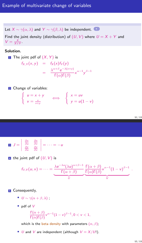
Let $f_{X_1,X_2}(x_1,x_2)$ be the joint density function of two continuous r.v.s $X_1$ and $X_2$.
Assume that the map $(x_1,x_2)\mapsto (y_2,y_2)$ where $$ \begin{cases} y_1 = g_1 (x_1, x_2) \\ y_2 = g_2 (x_1, x_2) \end{cases} $$
has a unique inverse function
$$ \begin{cases} x_1 = h_1(y_1,y_2) \\ x_2 = h_2(y_1,y_2) \end{cases} $$
Then $Y_1 = g_1(X_1,X_2)$ and $Y_2 = g_2(X_1,X_2)$ are jointly continuous with joint density function givenby
$$ f_{Y_1,Y_2}(y_1,y_2) = f_{X_1,X_2}(h_1(y_1,y_2), h_2(y_1,y_2)) |J| $$
where
$$ J = \left| \begin{matrix} \frac{\partial x_1}{\partial y_1} & \frac{\partial x_1}{\partial y_2} \\ \frac{\partial x_2}{\partial y_1} & \frac{\partial x_2}{\partial y_2} \end{matrix} \right| = \frac{\partial x_1}{\partial y_1} \frac{\partial x_2}{\partial y_2} - \frac{\partial x_1}{\partial y_2} \frac{\partial x_2}{\partial y_1} $$
???
Order Statistics
Let $X_1, X_2, \cdots, X_n$ be a i.i.d. sample of continuous r.v.'s with common cdf $F(x)$ and pdf $f(x)$.
The order statistics associated to the sample are the list of their sorted values $(X_{(1)}, X_{(2)}, \cdots, X_{(n)})$, where
$$ X_{(1)} < X_{(2)} < \cdots < x_{(n)} $$
Theorem: For $1 \le i \le n$, the $i$-th order statistic $X_{(i)}$ has pdf
$$ f_{(i)}(x) = \frac{n!}{(n-i)!(i-1)!} f(x) (F(x))^{i-1} (1-F(x))^{n-i} $$
Theorem: Jointly, the $n$ order statistics has pdf
$$ f_{(1,2,\cdots,n)}(x_1,x_2, \cdots, x_n) = n! \prod_{i=1}^n f(x_i), \quad x_1 < x_2 < \cdots < x_n $$
Conditonal Expectation
Conditional expectation of $X$ given that $Y=b$: Sipmly, defined to be the mean of the conditional distribution $f_{X|Y}(X|Y=b)$ i.e.
$$ E[X|Y=b] = \int x \cdot p_{X|Y}(x|b) $$
Conditional expectation of $\varphi(X)$ given that $Y=b$: Similarly, this is mean of $\varphi(X)$ under the conditional distribution $p_{X|Y}(\varphi(X)|Y=b)$ i.e.
$$ E(\varphi(X)|Y=b) = \int \varphi(x) \cdot p_{X|Y} (x|b) $$
Part 2 Markov Chains
2.1 Introduction
An example: Random Walk
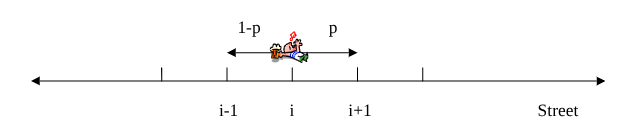
A drunkard in midnight on a endless street, he can't control himself and has a probability $p$ to go ahead and $1-p$ to turn back.
A mathematical representation of the random walk. Let $X_0$ be the starting point and $Y_n$ be the $n$-th step taken:
$$ Y_n = \begin{cases} +1, \quad & \text{with probability }p, \\ -1, \quad & \text{with probability }1-p \end{cases} $$
Then $\{Y_n, n=1,2,\cdots\}$ are i.i.d. rvs and the position at time $n$ (or after $n$ steps) is just
$$ X_n = Y_0 + Y_1 + \cdots + Y_n $$
Starting point: $X_0=i_0$. At time $n$, where will he go next step?
Definition: A discrete state space stochastic process $\{X_n\}_{n \ge 0}$ is a Markov Chain (MC) if
$$ P(X_{n+1}=j | X_n=i, X_{n-1} = i_{n-1}, \cdots, X_1 = i_1, X_0 = i_0) = P(X_{n+1}=j | X_n = i) $$
for all states $i_0, i_1, \cdots, i_{n-1}, i, j$ and all $n \ge 0$.
左边的式子是:已知现在在 $i$,而且知道从 $0$ 时刻到现在的全部历史,那么下一步去 $j$ 的概率是多少?
右边的式子是:只知道现在在 $i$,下一步去 $j$ 的概率是多少?
那么如果这两个概率永远相同,那么就是 Markov Chain。Markov 不一定意味着现实真的没有记忆,而是你的“状态”必须包含预测未来所需的全部信息。
We consider homogeneous MC only: $P(X_{n+1} = j | X_n = i) = p_{ij}$ is independent from the time $n$.
Meaning of the Markov property: Past, Present and the Future states
$$ \underbrace{X_{n+1}}_{\text{future}} \qquad \underbrace{X_n}_{\text{present}} \qquad \underbrace{X_{n-1},\ldots,X_1,X_0}_{\text{past}} $$
Markov Property: 'future' states depend only on 'present' states and not on 'past' states:
$$ P(\text{future}|\text{present}, \text{past}) = P(\text{future}|\text{present}) $$
Transition Probabilities:
One-step transition probabilities:
$$ p_{ij} = P(X_{n+1}=j | X_n=i) $$
$p_{ij}$: The probability that the process will, when in state $i$, next make a transition into state $j$.
$p_{ij}$ 表示现在在状态 $i$,下一步跑到状态 $j$ 的概率是多少?
For any $i$, the family $p_i=\{j \mapsto p_{ij}\}$ is the conditional distribution of $X_{n+1}$ given $X_n=i$; in particular $p_{ij} \ge 0$, and for all $j$, $\sum_{j=0}^\infin p_{ij}=1$
One-step transition matrix of the Markov Chain is the matrix:
$$ P = (p_{ij}) = \begin{pmatrix} p_{00} & p_{01} & \cdots & p_{0j} & \cdots \\ p_{10} & p_{11} & \cdots & p_{1j} & \cdots \\ \vdots & \vdots & \vdots & \vdots & \vdots \\ p_{i0} & p_{i1} & \cdots & p_{ij} & \cdots \\ \vdots & \vdots & \vdots & \vdots & \vdots \end{pmatrix} $$
e.g. Consider $2$ states of weather:
$$ X_i = \begin{cases} 0, \quad \text{Sunshine} \\ 1, \quad \text{Rainy} \end{cases} $$
Suppose we have the matrix
$$ P = \begin{pmatrix} 0.8 & 0.2 \\ 0.4 & 0.6 \end{pmatrix} $$
And consider
$$ p_{00}=0.8=P(X_{n+1}=0 | X_n = 0) $$
represents if today is sunshine, then the probability of tomorrow is sunshine is $0.8$.
And $p_{01}=0.2$ represents if today is sunshine, then the probability of tomorrow is rainy is $0.2$.
e.g. Now look back at the drunkard's random walk:

$$ P = (p_{ij}) = \begin{pmatrix} \vdots & \ddots & \vdots & \vdots & \vdots & \vdots & \vdots \\ \cdots & 1-p & 0 & p & \cdots & \cdots & \cdots \\ \cdots & 0 & 1-p & 0 & p & \cdots & \cdots \\ \vdots & \vdots & \vdots & \vdots & \ddots & \vdots & \vdots \end{pmatrix} $$
Important Properties
Joint Distribution: For a MC with transition probabilities $\{p_{ij}\}$,
$$ P(X_n = i_n, \cdots, X_1 = i_1, X_0 = i_0) = P(X_0 = i_0) \cdot \prod_{i=0}^{n-1} p_i p_{i+1} $$
for $n \ge 1$ and $(i_0,i_1, \cdots, i_n) \in E^{n+1}$
一条具体路径发生的概率 $=$ 起点概率 $\times$ 每一步转移概率
Conditional Probabilities
For any $n > k_1 > k_2 > \cdots > k_m > 0$
$$ P(X_n = i_n | X_{k_1} = i_{k_1}, X_{k_2} = i_{k_2}, \cdots, X_{k_m} = i_{k_m}) = P(X_n = i_n | X_{k_1} = i_{k_1}) $$
已知离 $n$ 最近的信息 $k_1$,那么剩下的都没用(依旧 Markov Property)
2.2 Chapman-Kolmogorov Equation
$n$-step Transition Probabilities $p_{ij}^{(n)}$
Definition: probability that a process in state $i$ will be state $j$ after $n$ additional transitions;
$$ p_{ij}^{(n)} = P(X_n = j | X_0 = i), \quad i,j \in E $$
从状态 $i$ 出发,走 $n$ 步以后到状态 $j$ 的概率
Chapman-Kolmogorov Equation
$$ p_{ij}^{(n+m)} = \sum_{k \in E} p_{ik}^{(n)} \cdot p_{kj}^{(m)}, \quad n, m \ge 0, i, j \in E $$
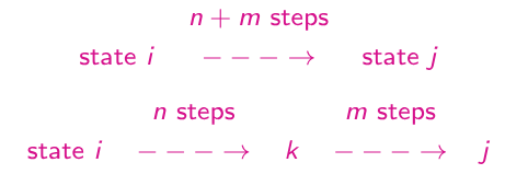
Put it in matrix form:
$$ P^{(n)} = \left( p_{ij}^{(n)} \right), P^{(n+m)} = P^{(n)} P^{(m)} $$
In particular, $P^{(n)} = P^{(n-1)} P = P\cdots P = P^n$
其实就是之前学过的矩阵乘法加速 DP 递推式子
Special Case: By convention for $n=0, P^0 = I$, the identity matrix. In other words,
$$ P_{ij}^{(0)} = P(X_0=j|X_0=i) = 1_{i=j} $$
Probability Distribution of $X_n$ at Time $n$
Matrix form: for $n \ge 0$, let $\mu=$ the p.m.f. of $X_n$ written as a row vector:
$$ \mu_n = (P(X_n=0), P(X_n=1), \cdots, P(X_n=i)) $$
Then,
$$ \begin{aligned} \mu_n(j) &= P(X_n=j) \\ &= \sum_{i \in E} P(X_{n-1}=i, X_n = j) \\ &= \sum_{i \in E} P(X_{n-1}=i) P(X_n = j | X_{n-1}=i) \\ &= \sum_{i \in E} \mu_{n-1} (i) p_{ij}, \quad j \in E \end{aligned} $$