MAT3007 Optimization
Prof. Yongchun Li
Three main subjects:
- Linear Optimization
- Disciplined linear programming
- Algorithms
- Duality
- Nonlinear Optimization
- Optimally condition
- Nonlinear optimization alorigthms
- Integer Optimization
- Baisc algorithms
- Assignments: 30%
- Midterm Exam(24 June): 30%
- Final Exam(18 July): 40%
Lecture 1
Brief Introduction
Common components of optimization problems:
- Decision 决策
- Objective 目标
- Constraints 限制条件
Optimization concerns choosing a decision(or decisions) to optimize certain objectives while subject to certain constraints.
最优化即选择一个决策(或一些决策)去最优化一些目标,在某些限制条件下。
Optimize could mean maximize or minimize depending on the problem contxt. 最大化 / 最小化
Optimization Problems
Mathematically, an optimization problem is usually represented as: $$ \begin{aligned} \min_{x} \quad & f(x) \\ \text{subject to} \quad & x \in \Omega \end{aligned} $$ where we have $x$ for Decision, $f$ for Objective funtion and $\Omega$ for Constraints.
In practice, we often consider a slightly more restrictive form: $$ \begin{aligned} \min_{x \in R^n} \quad & f(x) \\ \text{subject to } \quad & g_i(x) \leq 0, \quad \forall i = 1, \cdots, m \\ \text{subject to } \quad & h_j(x) = 0, \quad \forall i = 1, \cdots, p. \end{aligned} $$ where $x \in R^n$ is Decision variables(a vector), $f(x)$ is Objecive funtion and $g(x) \leq 0, h(x) = 0$ is Inequality and equality constraints. $$ g(x) = \begin{bmatrix} g_1(x) \\ \vdots \\ g_m(x) \end{bmatrix} \in R^m \text{ and } h(x) = \begin{bmatrix} h_1(x) \\ \vdots \\ h_p(x) \end{bmatrix} \in R^p $$ We can also express the constraints using the abstarct format: $$ \begin{aligned} \Omega &:= \{x \in R^n: g_i(x) \leq 0, i = 1, \dots, m, h_j(x) = 0, j = 1, \dots, p \} \\ &= \{x \in R^n: g(x) \leq 0, h(x) = 0 \} \end{aligned} $$
Feasible point: A decition that satisfies all constraints. 可行点
Feasible region(set) $\Omega$: The set of all feasible points.
Optimal solution:
Optimal value
Minimizer 最优解
Let $\Omega \subseteq R^n$ be a nonempty set and let $f : \Omega \to R$ be given. We define $$ B_{\epsilon(y)} := \{x \in R^n: \Vert x-y \Vert < \epsilon \} $$ to be the open ball(开球) in $R^n$ with center $y$ and radius $\epsilon > 0$
The point $x^* \in R^n$ is said to be a:
- Local minimizer(局部最优解)
- Strict local minimizer(严格局部最优解)
- Global minizer(全局最优解)
- Strict global minimzer(严格全局最优解)
Remark: global minimizer = global solution = optimal solution
Properties of Optimization Problems
Some facts:
- The feasible set can be empty(infeasible).
- An optimization problem may not always have an optimal solution.
- The optimal value can be unbounded.
- Even if an opt. problem is feasible, finite, and can attain its optimal value, the optimal solution may not be unique.
By classifying the different outcomes, an opt. problem may have the following stats:
- Infeasible
- Feasible, optimal value finite but not attainble.
- Feasible, optimal value finite and attainable.
- Feasible, but optimal value is unbounded.
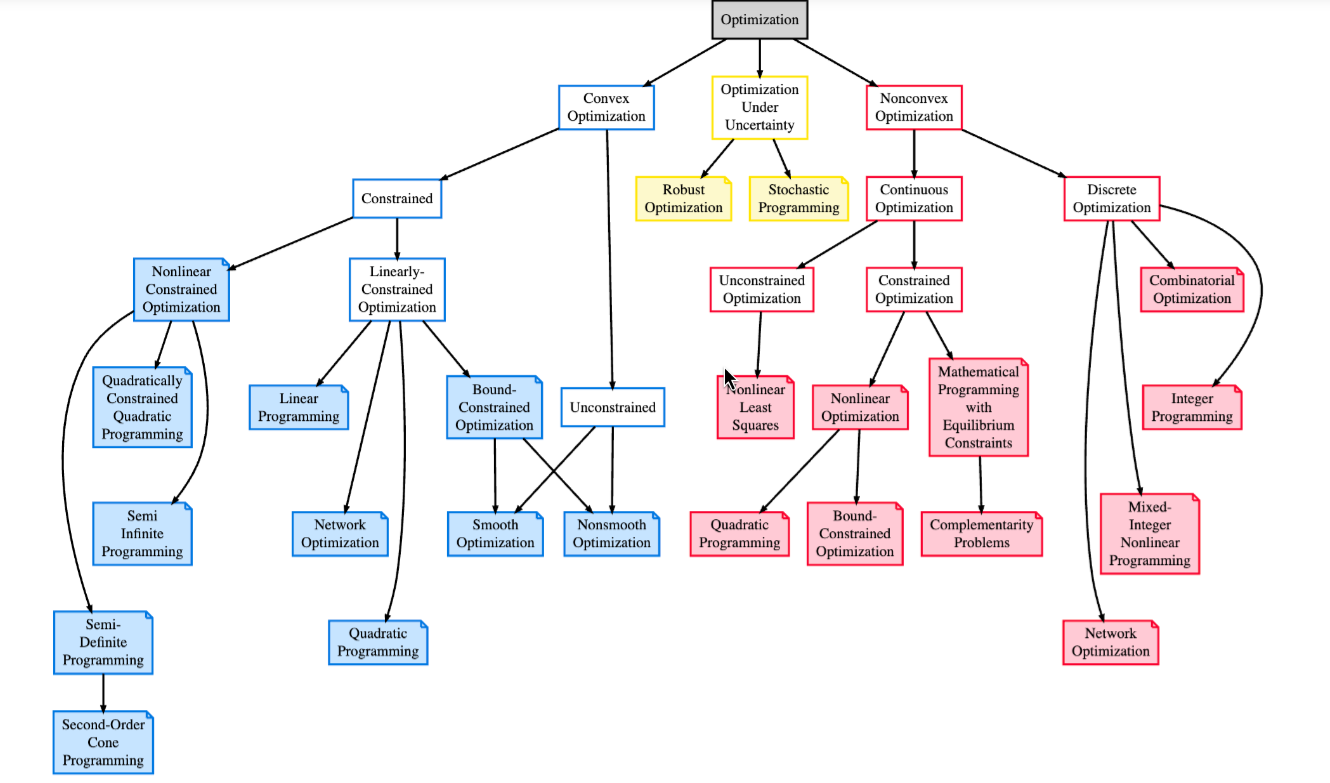
Classifications of Optimization
Unconstrained optimization: If $m = p = 0$. Otherwise constrained optimization.
Linear Programming(LP): Constraints and objective function are linear in the decision variables.
Nonlinear Programming(NLP): Either some of the constraints or the objective funtion if nonlinear.
Convex Optimization: If $f(x)$ and all $g_i(x)$ and convex, and $h_j(x)$ are linear (i.e. the feasible set is convex).
Integer Programming(IP): Some of the decision variables have to be integers.
Modeling 建模
e.g. Maximum Area Problem.
You have 80 meters of fencing and want to enclose a rectangular area - as large as possible.
- Decision variable: the length $l$ and width $w$ of the area.
- Objective: maximize the area: $lw$
- Constraints: the total length of the fence: $2l + 2w \leq 80$
Therefore, the optimization problem can be written as $$ \begin{aligned} \max_{l, w} \quad & lw \\ \text{subject to} \quad & 2l+2w \leq 80 \ & l, w \geq 0 \end{aligned} $$
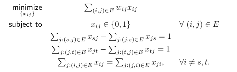
e.g. Shortest Path Problem
Set of notdes $V$, set of edges: $E \subset V \times V$. The distance between node $i$ and node $j$ is $w_{ij}$.
For each edge $(i, j) \in E$, define $$ x_{ij} = \begin{cases} 1 , & \text{if we use edge }(i,j), \\ 0 , & \text{otherwise}. \end{cases} $$
Directed graph: $x_{ij}$ does not necessarily equal to $x_{ji}$. And we have the following optimization modeling
Lecture 2
Linear Programming 线性规划
Def. A linear optimization or linear programming(LP) problem is an optimization problem in which the objective function and all constraint functions are linear (in the decision variables)
e.g. $$ \begin{aligned} \max_{x_1, x_2, x_3} \quad & f(x) = 40 x_1 + 30 x_2 + 50 x_3 \\ \text{subject to} \quad & x_1 + x_2 + x_3 \leq 100 \\ & 2x_1 + x_2 + 3x_3 \leq 180 \\ & x_3 \geq x_1 \\ & x_1, x_2, x_3 \geq 0 \end{aligned} $$
General Formulation
$$ \begin{aligned} \min_{x \in R^n} \quad & c^\top x \\ \text{subject to} \quad & a_i^\top x \geq b_i \quad &\forall i \in m_1 \\ & a_i^\top x \leq d_i \quad &\forall i \in m_2 \\ & a_i^\top x = e_i \quad &\forall i \in m_3 \\ & x_i \geq 0 \quad &\forall i \in n_1 \\ & x_i \leq 0 \quad &\forall i \in n_2 \\ & x_i \text{ free} \quad &\forall i \in n_3 \end{aligned} $$
where $m_1, m_2, m_3$ are subsets of $\{1, \dots, m\}$, $n_1, n_2, n_3$ are subsets of $\{1, \dots, n\}$.
Standard Form of LPs
An LP is said to be of the standard form if it is of the form: $$ \begin{aligned} \min_{x \in R^n} \quad & c^\top x \\ \text{subject to} \quad & Ax = b \\ & x \geq 0 \end{aligned} $$
where $x \in R^n$, $A$ is an $m \times n$ matrix($m < n$), and $b \in R^m$.
Any LP can be written in the standard form, using "tricks".
Standard From Transformations:
- Maximization: use $-c$ instead of $c$ to change it to minimization.
- Eliminating inequality constraints using slack variables $s$.
- $Ax \leq b \Rightarrow Ax+s=b, s \geq 0$
- $Ax \geq b \Rightarrow Ax-s=b, s \geq 0$
- If one has $x_i \leq 0$, replace $x_i$ by $-y_i$ and add $y_i \geq 0$
- Eliminating free variables $x_i$ (no constraints on $x_i$) by replacing $x_i$ by $x_i^+ - x_i^-$, where $x_i^+ \geq 0, x_i^- \geq 0$
e.g.
Consider a LP problem: $$ \begin{aligned} \max \quad & 3x_1 - 2x_2 + x_3 \\ \text{subject to} \quad & 2x_1 + 3x_2 + 4x_3 \geq 1 \\ & 3x_1 + 4x_2 \leq 5 \\ & 5x_2 - x_3 = -1 \\ & x_1, x_2 \geq 0 \end{aligned} $$
We can transform it into standard form: $$ \begin{aligned} \min \quad & -3x_1 + 2x_2 - x_3^+ + x_3^- \\ \text{subject to} \quad & 2x_1 + 3x_2 + 4x_3^+ - 4x_3^- - x_4 = 1 \\ & 3x_1 + 4x_2 + x_5 = 5 \\ & 5x_2 - x_3^+ + x_3^- = -1 \\ & x_1, x_2, x_3^+, x_3^-, x_4, x_5 \geq 0 \end{aligned} $$
More Modeling
Minimax Objective Problem: $$ \begin{aligned} \min_x \quad & \max_{i=1,\cdots,n} \{ c_i^\top x + d_i \} \\ \text{subject to} \quad & Ax=b \\ & x \geq 0 \end{aligned} $$
Solution: define $y = \max_{i=1,\cdots,n} \{ c_i^\top x + d_i \}$ and consider: $$ \begin{aligned} \min_{x,y} \quad & y \\ \text{subject to} \quad & y \geq c_i^\top x + d_i \\ & Ax=b \\ & x \geq 0 \end{aligned} $$
Minimizing Absolute Values $$ \begin{aligned} \min_x \quad & \sum_{i=1}^n \lvert x_i \rvert \\ \text{subject to} \quad & Ax=b \\ \end{aligned} $$ This can be equivalently written as: $$ \begin{aligned} \min_{x,t} \quad & \sum_{i=1}^n t_i \\ \text{subject to} \quad & x_i \leq t_i \\ & x_i \geq -t_i \\ & Ax=b \end{aligned} $$
A Modeling Tool
Consider the optimization problem: $$ \begin{aligned} \min_{x} \quad & \sum_{i=1}^m f_i(x) \\ \text{subject to} \quad & x \in \Omega \end{aligned} $$ It is equivalent to $$ \begin{aligned} \min_{x,t} \quad & \sum_{i=1}^m t_i \\ \text{subject to} \quad & x \in \Omega \\ & f_i(x) \leq t_i \end{aligned} $$ Where $f_i: R^n \to R$ are given and $\Omega \subset R^n$ is the feasible set.
Lecture 3
Solving Linear Programming Graphically
Recall the production problem: $$ \begin{aligned} \max \quad & x_1 + 2x_2 \\ \text{subject to} \quad & x_1 \leq 100 \\ &2x_2 \leq 200 \\ &x_1 + x_2 \leq 150 \\ &x_1, x_2 \geq 0 \end{aligned} $$
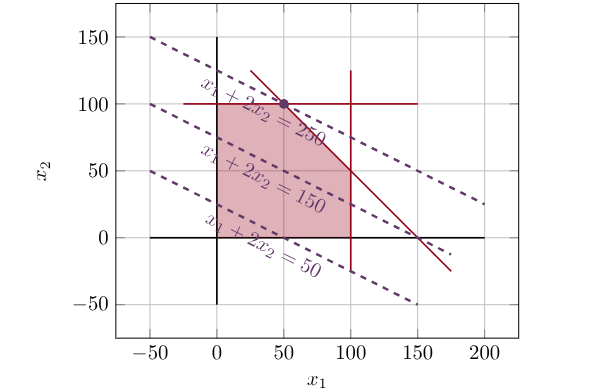
The red polygon is the feasible region.
And the optimal solution is the highest one among these lines that touches the feasible region.
Some Obeservations:
- The feasible region of an LP is a polyhedron 多面体
- The optimal solution tends to be a vertex/corner of the feasible region.
- Some constraints are active at the optimal solution, some are inactive
Def. A Polyhedron is a set that can be written in the form $$ \{ x \in R^n: Ax \geq b \} $$ where $A$ is an $m \times n$ matrix and $b \in R^m$.
注:这里的 Polyhedron 多面体,并不是传统意义上的三维多面体,而是可以有更高维度的多面体,无法直观现象。
Def. Convex Set: A set $S \subseteq R^n$ is convex if $$ \forall x, y \in S \\ \forall \lambda \in [0,1], \lambda x + (1- \lambda) y \in S $$
Def. Convex Combination: For any $x_1, \cdots, x_n$ and $\lambda_1 + \cdots + \lambda_n = 1$, we call $\sum_{i=1}^n \lambda_i x_i$ a convex combination of $x_1, \cdots, x_n$.
Def. Exetreme Point: Let $P$ be a polyhedron. A point $x \in P$ is said to be an extreme point of $P$ if we cannot find two elements $y,z \in P$ with $y,z \not= x$ and a scalar $\lambda \in [0,1]$, such that $x = \lambda y + (1-\lambda) z$.
Consider the production problem example above, it has $5$ exetreme points.
Exetreme Points and Basic Feasible Solutions
Consider an LP in its standard form: $$ \begin{aligned} \min_{x \in R^n} \quad & c^\top x \\ \text{subject to} \quad & Ax = b \\ & x \geq 0 \end{aligned} $$ where $x \in R^n$, $A$ is an $m \times n$ matrix($m < n$), and $b \in R^m$.
General Assumption: $A$ has linearly independent rows (or equivalently $A$ hass full row rank $m$)
Def. Basic Solution: We call $x$ a basic solution(BS) of the standard form LP iff:
- $Ax = b$
- There exist indices $B(1), \cdots, B(m)$ such that the columns of $$ \begin{bmatrix} | & | & & | \\ A_{B(1)} & A_{B(2)} & \cdots & A_{B(m)} \\ | & | & & | \end{bmatrix} $$ are linear independent and $x_i=0$ for $i \not= B(1), \cdots, B(m)$.
Finding a Basic Solution
Procedure:
- Choose any $m$ independent columns of $A$: $A_{B(1)}, \cdots, A_{B(m)}$
- Let $x_i=0$ for all $i \not= B(1), \cdots, B(m)$.
- Solve the equation $Ax=b$ for the remaining $x_{B(1)}, \cdots, x_{B(m)}$, giving $x_B = A_B^{-1} b$
Since $A_{B(1)}, \cdots, A_{B(m)}$ are linearly independent, the last step must produce a unique solution. Basic solution of an LP only depends on its constraints, it has nothing to do with the objective function.
Basic Feasible Solutions
Def. If a basic solution $x$ also satisfies that $x \geq 0$, then we call it a basic feasible solution (BFS).
Example
Still production problem...
$$
\begin{aligned}
\max \quad & x_1 + 2x_2 \\
\text{subject to} \quad & x_1 \leq 100 \\
&2x_2 \leq 200 \\
&x_1 + x_2 \leq 150 \\
&x_1, x_2 \geq 0
\end{aligned}
$$
with standard form:
$$
\begin{array}{rlrrrrrrl}
\min & -x_1 & & -2x_2 & & & & & \\
\text{subject to} & x_1 & & & & +s_1 & & & = 100 \\
& & & 2x_2 & & & & +s_2 & = 200 \\
& x_1 & & +x_2 & & & &+ s_3 & = 150 \\
& x_1, & & x_2, & & s_1, & & s_2, \quad s_3 & \ge 0
\end{array}
$$
We can denote the fesibale set by $\{ x:Ax=b, x \geq 0 \}$ where
$$
A =
\begin{bmatrix}
1 & 0 & 1 & 0 & 0 \\
0 & 2 & 0 & 1 & 0 \\
1 & 1 & 0 & 0 & 1
\end{bmatrix}, \quad
b =
\begin{bmatrix}
100 \\
200 \\
150
\end{bmatrix}
$$
We can choose three independent columns of $A$, e.g. the first three $(B = \{1, 2, 3\})$, we get the corresponding basic solution via:
$$
x_B =
\begin{bmatrix}
1 & 0 & 1 \\
0 & 2 & 0 \\
1 & 1 & 0
\end{bmatrix}^{-1}
\begin{bmatrix}
100 \\
200 \\
150
\end{bmatrix} =
\begin{bmatrix}
50 \\
100 \\
50
\end{bmatrix}
$$
That is $x_1 = 50, x_2 = 100, s_1 = 50$, therefore $(50, 100, 50, 0, 0)$ is a basic feasible solution.
One can find other basic feasible solution by choosing other sets of columns.
Extreme Points and BFS
For the standard LP polyhedron $\{ x:Ax=b, x \geq 0 \}$, we have:
$x$ is an extreme point $\Leftrightarrow$ $x$ is a basic feasible solution.
就是说,我们的可行解可以组成一个多面体,这个多面体的极值点(也就是顶点)其实就是 BFS,即通过组合矩阵 $A$ 里面的列组成满秩矩阵得到的解,作为端点,形成的多面体。
为什么满秩矩阵接出来的解即这个多面体的顶点?本质上可以理解为同时选了几个约束都到了极值点,那自然就形成了可行解的顶点。
Fundamental Theorem of LP
Fundamental LP Theorem: Consider a linear problem in standard form and assume that $A$ has full row rank $m$.
- If the feasible set is nonempty, there is a basic feasible solution.
- If there is an optimal solution, there must be at least one optimal solution that is also a basic feasible solution.
Corollary: Characteristics: If an LP with $m$ constraints (in the standard form) has an optimal solution, then there must be an optimal solution with no more than $m$ positive entries.
Lecture 4
The Simplex Method 单纯形法
Idea: The simplex method preceeds from one BFS (an extreme point of the feasible region) to a neighboring / adjacent one to continuously imporve the value of the object funtion until reaching optimality.
It usually talks on standard form LP: $$ \begin{aligned} \min_{x} \quad & c^\top x \\ \text{subject to} \quad & Ax=b \\ & x \geq 0 \end{aligned} $$
Neighboring BFS
Def. Neighboring Basic Solutions: Two basic solutions are neighboring / adjacent if they differ by exactly one baic (or non-basic) index.
e.g. A BFS constructed by using $B=\{ 1,2,3 \}$ is a neighbor to $B=\{ 1,3,5 \}$, but not a neighbor to $B=\{ 1,4,5 \}$
So if we consider checking all the neighbors of a BFS, which consists $m(n-m)$ potential neighbors, it likely to be very slow.
Finding a Neighboring BFS
First, we assume that we have somehow found a BFS whose basis is $B=\{ B(1),\cdots,B(m) \}$, and define: $$ \begin{bmatrix} | & | & & | \\ A_{B(1)} & A_{B(2)} & \cdots & A_{B(m)} \\ | & | & & | \end{bmatrix} $$ And let $A_N$ be the matrix consisting of the non-basic columns of $A$. We have $$ |B| = m, |N|=n-m \\ B \cup N = \{1,2,\cdots,n\} $$ We can write $$ A=[A_B, A_N], x=[x_B;x_N] $$ By definition, we have $$ x_B = A_B^{-1}b \quad x_N = 0 $$
To find a neighbor, we want to select a non-basic variable $x_j, j \in N$ to enter the basis. Which means we want to increase $x_j$ from the current BFS.
Basic Direction
We consider moving $x$ to a neighboring one $y$ by $$ y=x+\theta d, \quad \theta \geq 0 $$ where
- $d_j=1$
- $d_{j'}=0$ for all other non-basic indices $j' \not= j \in N$.
We need to guarantee that the resulting step $y=x+\theta d$ is still feasible, that is: $$ A(x+\theta d) = b = Ax $$ i.e. $Ad=0$
Now, we write $d=[d_B;d_N]$, since $d_j=1$ and $d_{j'}=0$ for all other non-basic indices, we have $$ 0= \begin{bmatrix} A_B & A_N \end{bmatrix} \begin{bmatrix} d_B \\ d_N \end{bmatrix}= A_B d_B + A_j $$ Therefore $$ d_B = -A_B^{-1}A_j $$ Which means the direction $d$ is uniquely determined once $j$ is chosen: $$ d=[d_B;d_N]=[-A_B^{-1}A_j;0;\dots;1;\dots;0] $$ where the $1$ is at the $j^{th}$ entry, we call such $d$ the $j^{th}$ basic direction.
简单来讲,就是我们现在站在一个 BFS(顶点)上,我们想要走到相邻顶点。我们选一个 non-basic 变量 $x_j$,让它从 $0$ 开始变大,且一直满足 $Ax=b$ 约束。
当 $x_j$ 增加时,basic 变量也必须跟着变化,来抵消 $x_j$ 对约束的影响,,其方向为 $d_B=-A_B^{-1}A_j$。然后沿着 $y=x+\theta d$ 走,直到某个 basic 变量变成 $0$,那这个变成 $0$ 的 basic 变量就会离开 basis。
至此,得到了一个新的 BFS。但是,朝着这个方向走,目标函数会变好吗(更优)?
Reduced Cost
The target function is
$$
c^\top x
$$
if walking $x$ to $y=x+\theta d$, the change of function will be
$$
\begin{aligned}
\Delta &= c^\top y-c^\top x \\
&= c^\top (x+\theta d)-c^\top x\\
&= \theta c^\top d
\end{aligned}
$$
We define the reduced cost
$$
\begin{aligned}
\bar{c}_j &= c^\top d \\
&= c_B^\top d_B + c_j \\
&= c_B^\top (-A_B^{-1}A_j)+c_j \\
&= c_j - c_B^\top A_B^{-1} A_j
\end{aligned}
$$
And in minimization problem, if a non-basic variable $x_j$'s reduced cost satisfies $\bar{c}_j < 0$, it means it will decrease the function (better direction) if it enters basis.
Thus simplex will choose a variable of $\bar{c}_j < 0$ to enter basis.
If all non-basic variables satisfy $\bar{c}_j \ge 0$, it means there is no neibouring that decrease the target function, and it is the Optimization Answer.
Theorem: Stopping Criterion
Consider a basic feasible solution $x$ associated with the basis $B(1), B(2), \cdots, B(m)$ and let $\bar{c} = [\bar{c}_1; \cdots; \bar{c}_n]$ be the corresponding vector of reduced costs. If $\bar{c}_j \ge 0$, then $x$ must be optimal.
这个比较好理解,就是不断找能使得目标函数更小的加入 Basis,顺便带走一个,直到找不到能替换的为止。
Choosing a Stepsize $\theta$
After choosing an entering variable, we know the direction $d$, but we still need to choose how far we can move along this direction while keeping feasibility.
The feasibility requires: $$ y = x + \theta d \ge 0 $$ For variables with $d_i \ge 0$, there is no restriction on $\theta$, but for variables with $d_i < 0$, we need $$ x_i + \theta d_i \ge 0 $$ $$ \theta \le -\frac{x_i}{d_i} $$ Therefore the largest feasible stepsize is: $$ \theta^* = \min_{i\in B, d_i <0} \left\{ -\frac{x_i}{d_i} \right\} $$
其实就是,沿着这个方向 $d$ 走,谁先变成 $0$,谁就限制了能走多远。
Consider the minimum number is reached by a basic variable $x_\ell$, we have $$ \theta^* = -\frac{x_\ell}{d_\ell} $$ $$ y_\ell = x_\ell + \theta^* d_\ell = 0 $$ That is, $x_\ell$ is leaving basis, and the entering variable $x_j$ is entering basis. The basis changed from $B$ to $B'=B-\{\ell\} + \{j\}$.
This is a simplex pivot.
What if no variable is decreasing?
If the direction satisfies $$ d \ge 0 $$ That is walking along the direction and all variables are not gonna be negative. $$ x + \theta d \ge 0 $$ Meanwhile since we are choosing $$ \bar{c}_j < 0 $$ So the target function is always decreasing, that is the LP has no limit optimal solution, which is unbounded.
Conclusion
Initialization: We start from a BFS $x$ with corresponding basis $B$.
-
We first compute the reduced costs $\bar{c}$: $$ \bar{c}_j = c_j - c_B^\top A_B^{-1} A_j $$
- If $\bar{c} \ge 0$, then $x$ is optimal.
- Otherwise choose some $j \in N$ such that $\bar{c} < 0$.
-
Compute the $j^{th}$ basic direction $d$ $$ d = [-A_B^{-1}A_j;0;\cdots;1;\cdots;0] $$
- If $d \ge 0$, then the problem is unbounded.
- Otherwise, compute $\theta^*$:
$$ \theta^* = \min_{i\in B, d_i <0} \left\{ -\frac{x_i}{d_i} \right\} $$
-
Set $y=x+\theta^* d$. Then the point $y$ is the new BFS with index $j$ replacing $B(\ell)$ in the basis. The objective function value (decrease) is changed by $$ \theta^* c^\top d = \theta^* \bar{c}_j $$
-
Repeate this procedures.
站在当前 BFS 上,用 reduced cost 找一个能让目标变好的 non-basic variable,让它进入 basis;然后沿着对应 basic direction 走,用 minimum ratio test 找最多能走多远;走到某个 basic variable 变成 $0$,让它离开 basis;得到新的 BFS;重复直到所有 reduced costs 都不能让目标变好。
Lecture 5
Degeneracy
Def. We call a BFS $x$ degenerate if some of the basic variables $x_B$ are $0$. Otherwise, it is non-degenerate.