MAT3350 Introduction to Information Theory
Prof. Kaiming SHEN @ SSE
Grades:
- Assignments / Quiz (20%)
- Midterm Exam (40%)
- Final Exam (40%)
Reference Book: T. Cover & J. Thomas: Elements of Information Theory 2nd Ed.
Chapter 1: Introduction 简介
1.1 Intergration of Information
Bit: $\{0, 1\}$
Information is the minimum number of bits ($0$ or $1$) to describe a random variable.
信息即用描述一个随机变量所使用 bits 的最小数量。
e.g. Weather Forecast
$$ X = \begin{cases} \text{rain}\ &50\% \ &0 , \\ \text{shine}\ &50\% \ &1 \end{cases} $$
From weatherman, we can learn value of $X$. And $X$ contains $1$ bit of information.
我们认为这个随机变量 $X$ 包含 $1$ bit 的信息。
假设我们现在有 $8$ 种不同的天气,每个概率相同,我们可以用 $X = \{000, 001, \cdots, 111\}$ 来表示天气。那么我们认为 $X$ 包含 $3$ bit 的信息,因为其最少可以用 $3$ 位 bit 来表示。
e.g. Horse Race (sp.)
$$ X = \begin{cases} A &\frac{1}{2} &000 &0 \\ B &\frac{1}{4} &001 &10 \\ C &\frac{1}{8} &010 &110 \\ D &\frac{1}{16} &\cdots &1110 \\ E &\frac{1}{64} &\cdots &111100 \\ F &\frac{1}{64} &\cdots &111101 \\ G &\frac{1}{64} &\cdots &111110 \\ H &\frac{1}{64} &\cdots &111111 \end{cases} $$
Information of $X=1 \times \frac{1}{2} + 2 \times \frac{1}{4} + 3 \times \frac{1}{8} + 4 \times \frac{1}{16} + 6 \times \frac{1}{64} \times 4 = 2 $ bits
1.2 Information Transmission over Channel
$$ X \rightarrow \text{Channel} \rightarrow Y $$
Channel: $P(y|x)$,就是一个条件概率,用来描述 $Y$ 是如何随着 $X$ 变化的。
Channel Capacity($C$) is the maximum number of bits that can be "reliably" transimitted from X to Y.
通道容量表示一个通信信道每次使用最多能够稳定传输多少信息。
1.3 Information Theory
Information Theory answers and questions:
-
What is the minimum number of bits to describe $X$?
Ans: Entropy $H(X)$ ... Data compression
-
What is the maximum numberof bits that can be reliably transmitted over channel?
Ans: Mutual info $I(X;Y)$ ... Channel Capacity.
Chapter 2: Entropy 熵
2.1 Basics
Def. Let $X$ be a discrete random variable, e.g. $X = \{a, b, c\}$, then: $$ X = \begin{cases} a, & p_1\\ b, & p_2\\ c, & p_3 \end{cases} $$ Which is easy to describe using probability mass function (PMF).
Def. The entropy of $X$ is $$ H(X) = \sum_x p(x) \log \frac{1}{p(x)} $$
When $\log$ is in base $2$, $H(X)$ is in "bit".
When $\log$ is in base $e$, $H(X)$ is in "nat".
$$ \log_e a = \ln a = \frac{\log_2 a}{\log_2 e} $$
$H(X)$ in nats $= \sum p(x) \log_e \frac{1}{p(x)} = \sum p(x) \left(\log_2 \frac{1}{p(x)}\right) \frac{1}{\log_2 e} = \frac{1}{\log_2 e} H(X)$ in bits.
Recall: $E[f(x)] = \sum_x p(x) f(x)$ (数学期望)
Note: $H(X) = E[\log{\frac{1}{p(x)}}] = -E[\log{p(x)}] $
Theorem: $H(X) \geq 0$
Proof: $0 \leq p(x) \leq 1 \Rightarrow \frac{1}{p(x)} \geq 1 \Rightarrow \log{\frac{1}{p(x)}} \geq 0 \Rightarrow H(X) \geq 0$
Theorem: Jensen's Inequality. For a $X = \{1, 2, \cdots, m\}$ $$ X = \begin{cases} 1, &p_1 \\ 2, &p_2 \\ \ \vdots \\ m, &p_m \end{cases} $$ We have $$ H(X) \leq \log m $$ Where "$=$" hold iff $X \sim \text{Uniform}$
And now we established the lower bound and upper bound of entropy: $$ 0 \leq H(X) \leq \log m $$
2.2 Connection to Data Compression
Shannon showed that $H(X)$ is the minimum number of bits to describe $X$. (will prove in the future)
e.g. $$ X = \begin{cases} 0 \quad 100\% \\ 1 \quad 0\% \end{cases} $$ And we can have: $$ \begin{aligned} H(X) = & 1 \times \log \frac{1}{1} + 0 \times \log \frac{1}{0} \\ = & 0 \end{aligned} $$ Since: $$ \lim_{x \to 0^+} x \log \frac{1}{x} = \lim_{x \to 0^+} -x \log x = \lim_{x \to 0^+} \frac{-\log x}{1/x} = \lim_{x \to 0^+}x = 0 $$
Another e.g.:
Consider $X_1, X_2, \cdots, X_{100}$. Each $X_i = \begin{cases}0 \quad 1 \% \\ 1 \quad 99 \% \end{cases}$
For a "typical" $(X_1, X_2, \cdots, X_{100})$, only one $X_i = 0$, rest are all $1$. $\Rightarrow$ Use $\log 100$ to describe $(X_1, X_2, \cdots, X_{100})$.
2.3 Connectoin to Computer Science
Def. Kolmogorov complexity $K(X)$ is the length of the shortest program that makes computer (Turing machine) print $X$.
e.g. $K(\pi) < \infty$
"Print $3.1415926\cdots$" has length $=\infty$
"Print the value between a circle circumference and its diameter" has lenght = $c$
这里可以理解为,虽然直接输出 $\pi$ 是无限的,但是一个生成 $\pi$ 的程序可以是有限的,即有$K(\pi) < \infty$
e.g. $K(101010\cdots10) \leq 2 + c'$
Suppose $10$ repeats $n$ times, "print $101010\cdots10$ has length $=2n+c$
But "print $10$ for $n$ times has length $=2\times 1 + c'$
Chapter 3: Condition Entropy
3.1 Basics
Recall: $H(X)$ is the minimum number of bits to describe $X$, which measures the uncertainty of $X$.
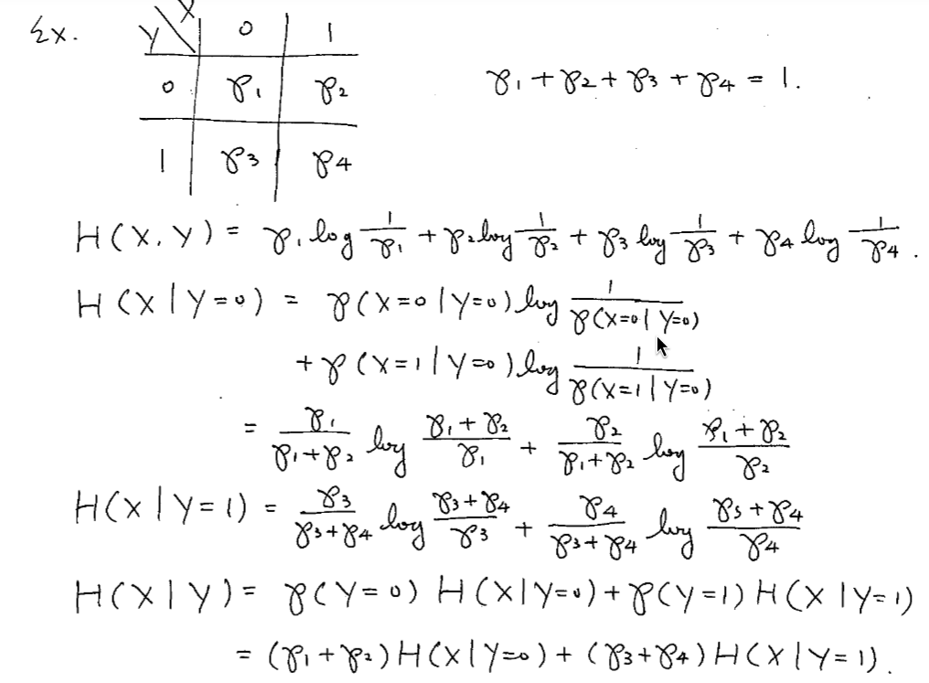
Def. For $(X,Y) \sim F(X,Y)$, the joint entropy: $$ \begin{aligned} H(X,Y) &= \sum_{(x, y)} p(x, y) \log \frac{1}{p(x, y)} \\ &= E\left[ \log \frac{1}{p(x,y)} \right] \end{aligned} $$ means the total uncertainty of $X$ and $Y$.
Def. Conditional entropy of $X$ with $Y$ known to be fixed at $y$ is: $$ \begin{aligned} H(X | Y=y) &= \sum_x p(x|y) \log \frac{1}{p(x|y)} \\ &= E_x \left[ \log \frac{1}{p(x|y)} \right] \end{aligned} $$ measures the remaining uncertainty of $X$ after knowing $Y=y$.
Def. Conditional entropy of $X$ with $Y$ known is: $$ \begin{aligned} H(X|Y) &= \sum_y H(X|Y=y) \cdot p(y) \\ &= \sum_{x, y} p(x,y) \log \frac{1}{p(x|y)} \end{aligned} $$ measures the remaining uncertainty of $X$ after $Y$ is known.
e.g.
3.2 Properties of $H(X|Y)$
Entropy Chain Rule: $$ H(X, Y) = H(Y) + H(X|Y) $$ Intuition: Total uncertainty of $(X,Y)=$ uncertatinty of $Y$ alone $+$ remaining uncertainty of $X$ after knowing $Y$.
这里的加号可以理解为:熵是信息量,分两步说,第一步先告诉他 $Y$ 是什么,即有 $H(Y)$ 个 bit,第二步是已经知道 $Y$ 的情况下,在告诉他 $X$ 是什么,即 $H(X|Y)$ 个 bit,两步获得的信息量是相加的
By symmetry, $H(X,Y) = H(X) + H(Y|X)$ is also correct.
Extension: Chain rule for joint entropy: $$ H(X_1, X_2, \cdots, X_n) = H(X_1) + H(X_2 | X_1) + H(X_3 | (X_1, X_2)) + \cdots + H(X_n | (X_1, X_2, \cdots X_{n-1})) $$
Theorem: If $X$ and $Y$ are independent (no overlay), then: $$ H(X, Y) = H(X) + H(Y) $$ And we have: $$ H(X|Y) = H(X) \Leftrightarrow X \text{ and } Y \text{ are independent} \\ H(X|Y) = H(Y) \Leftrightarrow X \text{ and } Y \text{ are independent} $$
3.3 Information never hurts
Theorem: Knowing $Y$ will not hurt our existing knowledge of $X$ $$ H(X|Y) \leq H(X) $$
So when in data compression, we can have:
e.g. Consider a probability table.
| $X\backslash Y$ | $0$ | $1$ |
|---|---|---|
| $0$ | $0.45$ | $0.05$ |
| $1$ | $0.05$ | $0.45$ |
And we have $$ X = \begin{cases} 0 \quad 50\% \\ 1 \quad 50\% \end{cases} $$
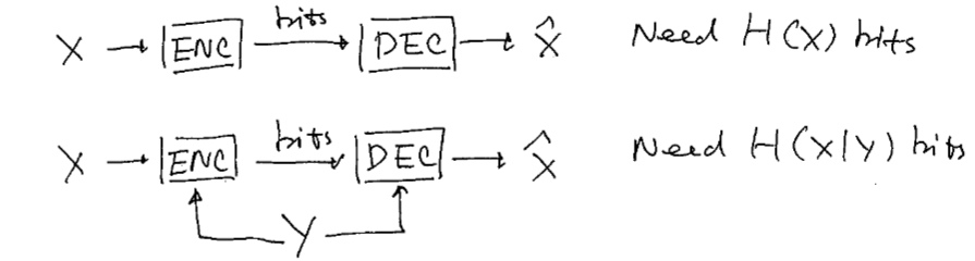
Without $Y$, we need $H(X) = 1$ bit to describe $X$.
Now $Y$ is provided, we can use the following equations: $$ X \oplus Y = Z \\ Y \oplus Z = X $$ Note that: $$ Z = \begin{cases} 0 \quad 90\% \\ 1 \quad 10\% \end{cases} $$ And we have $H(Z) < H(X)$, so the main idea is compressing $Z$ instead of $X$, and then recover $X$ with XOR.
e.g.
Consider $n$ balls, one ball is odd in that it is lighter or heavier than any other ball. Giving only one balance to compare two balls each time. How many times do we need to figure out which ball is odd?
Chapter 4: Mutual Information
4.1 Basics
Def. Mutual Information $$ \begin{aligned} I(X; Y) &= H(X) - H(X|Y) \\ &= H(X) + H(Y) - H(X, Y) \\ &= \sum_{x, y} p(x, y) \log \frac{p(x,y)}{p(x)p(y)} \\ &= E_{x,y} \left[ \log \frac{p(x,y)}{p(x)p(y)} \right] \\ \end{aligned} $$
Consider X -> Channel -> Y, then $I(X;Y)$ is the maximum number of bits reliably transmitted by our channel.
Now consider the venn graph below:

We have $$ \begin{aligned} &H(X|Y) = A \\ &H(Y|X) = C \\ &I(X;Y) = B \\ &H(X) = A+B \\ &H(Y) = B+C \\ &H(X, Y) = A+B+C \end{aligned} $$
4.2 KL Divergence
Def. For two distributions $p(x), q(x)$, their KL Divergence: $$ D(p || q) = \sum_x p(x) \log \frac{p(x)}{q(x)} $$
$D(p || q)$ gives "distance"(or "difference") between $p$ and $q$. BUT $D(p||q) \not= D(q||p)$
Def. Cross Entropy $$ CE(p,q) = \sum_x p(x) \log \frac{1}{q(x)} $$
Theorem: $$ CE(p,q) = H(p) + D(p||q) $$
CE(交叉熵)其实就是,比如在机器学习中,模型的理解 $q$ 和真实世界 $p$ 差得有多远,真实世界按照 $p$ 产生数据,但我用模型 $q$ 去预测它,平均会有多惊讶(可以作为 loss)
KL Divergence(KL 散度)就是因为用了错误模型 $q$,额外多付出了多少代价
4.3 Hypothesis Testing
Let $X_1, X_2, \cdots, X_n$ be independent random variables, but not sure which is their distribution, $p(x)$ or $q(x)$?
Two hypothesis:
- $H_1: X_i \sim p(x)$
- $H_2: X_i \sim q(x)$
Q: How to use $X_1, X_2, \cdots, X_n$ to decide which is true?
A: If $p(x)$ is more likely to produce $X_1, X_2, \cdots, X_n$, then $H_1$ is true, otherwise $H_2$ is true.
Def. Log-likelihood Ratoi: $$ LLR = \frac{1}{n} \log \frac{p(x_1, x_2, \cdots, x_n)}{q(x_1, x_2, \cdots, x_n)} $$ So the hypothesis test is:
- If $LLR > 0$, $p(x)$ will be the distribution
- If $LLR < 0$, $q(x)$ will be the distribution
Chapter 5: Conditional Mutual Information
5.1 Basics
Def. For $(X,Y,Z) \sim p(x,y,z)$, the conditional mutual information is $$ I(X;Y|Z)=H(X|Z)-H(X|Y,Z). $$
Equivalent forms: $$ \begin{aligned} I(X;Y|Z) &=H(Y|Z)-H(Y|X,Z) \\ &=H(X|Z)+H(Y|Z)-H(X,Y|Z) \\ &=H(X,Z)+H(Y,Z)-H(Z)-H(X,Y,Z). \end{aligned} $$
Interpretation:
- $H(X|Z)$: uncertainty of $X$ after side information $Z$ is known.
- $I(X;Y|Z)$: additional information about $X$ learned from $Y$ after $Z$ is already known.
先知道 $Z$,再看 $Y$。$I(X;Y|Z)$ 问的是:在已经知道 $Z$ 的情况下,$Y$ 还能额外告诉我们多少关于 $X$ 的信息。
Theorem: $$ I(X;Y|Z)\geq 0. $$ Equality holds iff $X$ and $Y$ are conditionally independent given $Z$: $$ p(x,y|z)=p(x|z)p(y|z). $$
Important warning: $$ I(X;Y|Z) $$ can be larger or smaller than $I(X;Y)$.
Example intuition:
- If $Z$ is pure noise independent of everything, conditioning on $Z$ does not help much.
- If $Z$ helps remove noise from $Y$, then $I(X;Y|Z)$ can become larger.
- If $Z$ already reveals $X$, then $I(X;Y|Z)=0$.
5.2 Chain Rule for Mutual Information
Theorem: $$ I(X_1,\cdots,X_n;Y) =I(X_1;Y)+I(X_2;Y|X_1)+\cdots+I(X_n;Y|X_1,\cdots,X_{n-1}). $$
Interpretation:
Instead of decoding all users together, we may decode one by one:
$$ (X_1,\cdots,X_n)\rightarrow \text{Channel}\rightarrow Y. $$
First decode $X_1$, then subtract the known part from $Y$, then decode $X_2$, and so on.
总信息量可以拆成“第一层信息 + 已知第一层后的第二层信息 + 已知前两层后的第三层信息 + ...”。
5.3 Markov Chain and Data Processing
Def. $X\to Y\to Z$ is a Markov chain if $$ p(x,y,z)=p(x)p(y|x)p(z|y). $$
Equivalently, $$ p(z|x,y)=p(z|y). $$
Intuition:
$$ X\to Y\to Z $$ means $Z$ depends on $X$ only through $Y$.
Theorem: If $X\to Y\to Z$, then $Z\to Y\to X$ is also a Markov chain.
Theorem: If $X\to Y\to Z$, then $X$ and $Z$ are conditionally independent given $Y$: $$ I(X;Z|Y)=0. $$
Theorem (Data Processing Inequality): If $$ X\to Y\to Z, $$ then $$ I(X;Z)\leq I(X;Y). $$
Also, $$ I(X;Z)\leq I(Y;Z). $$
信息经过处理不会凭空变多。$X$ 先告诉 $Y$,$Y$ 再告诉 $Z$,所以 $Z$ 对 $X$ 的了解不可能超过 $Y$ 对 $X$ 的了解。
Useful identity for proof: $$ I(X;Y,Z)=I(X;Z)+I(X;Y|Z) =I(X;Y)+I(X;Z|Y). $$
For Markov chain $X\to Y\to Z$, since $I(X;Z|Y)=0$, $$ I(X;Z)+I(X;Y|Z)=I(X;Y). $$
Chapter 6: Three-Party Mutual Information
6.1 Basics
Def. For $(X,Y,Z)\sim p(x,y,z)$, the three-party mutual information is $$ I(X;Y;Z)=I(X;Y)-I(X;Y|Z). $$
Equivalent forms: $$ \begin{aligned} I(X;Y;Z) &=H(X)+H(Y)+H(Z) \\ &\quad -H(X,Y)-H(X,Z)-H(Y,Z)+H(X,Y,Z). \end{aligned} $$
Symmetric identities: $$ I(X;Y;Z)=I(X;Z)-I(X;Z|Y)=I(Y;Z)-I(Y;Z|X). $$
Important warning: $$ I(X;Y)\geq 0,\qquad I(X;Y|Z)\geq 0, $$ but $$ I(X;Y;Z) $$ can be positive, zero, or negative.
two-party MI 和 conditional MI 都不会负;three-party MI 不一样,它不是一个普通的“信息量”,而更像三者重叠关系的代数量。
6.2 Information Theoretic Security
Let
- $X$ be plaintext,
- $K$ be key,
- $Y$ be ciphertext.
Encryption: $$ Y=f(X,K). $$
Decryption: $$ \hat X=g(Y,K). $$
Def. A system has perfect secrecy if $$ I(X;Y)=0. $$
This means the ciphertext reveals nothing about the plaintext without the key.
Def. The system is perfectly decodable if $$ H(X|Y,K)=0. $$
This means once both $Y$ and $K$ are known, $X$ can be recovered exactly.
Example (One-Time Pad):
Let $$ X\sim \operatorname{Bern}\left(\frac12\right),\qquad K\sim \operatorname{Bern}\left(\frac12\right) $$ independently, and define $$ Y=X\oplus K. $$
Then $$ \hat X=Y\oplus K. $$
So $$ I(X;Y)=0,\qquad H(X|Y,K)=0. $$
Theorem (Shannon's Perfect Secrecy Limit): If $$ I(X;Y)=0 $$ and $$ H(X|Y,K)=0, $$ then $$ H(K)\geq H(X). $$
想做到完全安全,key 的不确定性至少要和 message 一样大。One-time pad 安全,但 key 必须和 plaintext 一样长,所以实际很不方便。
Chapter 7: Entropy Rate
7.1 Motivation
For iid random variables $X_1,\cdots,X_n$, $$ H(X_1,\cdots,X_n)=\sum_{i=1}^n H(X_i)=nH(X_1). $$
But natural language, music, text, etc. are not iid. Later symbols depend on previous symbols.
Def. For a stochastic process $\mathcal X={X_i}$, the entropy rate is $$ H(\mathcal X)=\lim_{n\to\infty}\frac1n H(X_1,\cdots,X_n), $$ if the limit exists.
Examples:
If $X_i$ are iid, then $$ H(\mathcal X)=H(X_1). $$
If $X_i=X_1$ for all $i$, then $$ H(\mathcal X)=\lim_{n\to\infty}\frac1n H(X_1)=0. $$
entropy rate 是“平均每个新符号还带来多少新信息”。如果后面全是重复,平均新信息趋近于 0。
7.2 Stationary Stochastic Process
Def. A stochastic process $\mathcal X={X_i}$ is stationary if shifting time does not change the joint distribution: $$ p(X_1,\cdots,X_n)=p(X_{1+k},\cdots,X_{n+k}) $$ for all $n,k$.
Theorem:
For stationary $\mathcal X={X_i}$, $$ \lim_{n\to\infty} H(X_n|X_1,\cdots,X_{n-1}) $$ exists.
Moreover, $$ H(\mathcal X) =\lim_{n\to\infty}\frac1n H(X_1,\cdots,X_n) =\lim_{n\to\infty}H(X_n|X_1,\cdots,X_{n-1}). $$
Key idea:
Let $$ a_n=H(X_n|X_1,\cdots,X_{n-1}). $$
For stationary processes, $a_n$ is non-increasing: $$ a_{n+1}\leq a_n. $$
Also, $$ H(X_1,\cdots,X_n)=\sum_{i=1}^n a_i. $$
So the average converges to the same limit.
7.3 Markov Process
Def. A stochastic process is Markov if $$ p(X_n|X_1,\cdots,X_{n-1})=p(X_n|X_{n-1}). $$
That is, the future depends on the past only through the present.
Theorem:
If $\mathcal X$ is stationary and Markov, then $$ H(\mathcal X)=H(X_2|X_1). $$
If the stationary distribution is $\pi_i$ and transition matrix is $P_{ij}$, then $$ H(\mathcal X) =\sum_i \pi_i H(P_{i,\cdot}) =-\sum_i\sum_j \pi_i P_{ij}\log P_{ij}. $$
Example:
If $$ X_{n+1}=aX_n+Z_n, $$ where $Z_n$ are iid and independent of the past, then $$ H(\mathcal X)=H(X_2|X_1)=H(Z_1). $$
给定 $X_n$ 后,$X_{n+1}$ 的不确定性只来自新的 noise $Z_n$。
Chapter 8: AEP
8.1 LLN and AEP
Theorem (Law of Large Numbers):
For iid $X_i\sim p(x)$, $$ \frac1n\sum_{i=1}^n X_i \to E[X] $$ in probability.
Theorem (Asymptotic Equipartition Property, AEP):
For iid $X_i\sim p(x)$, $$ -\frac1n\log p(X_1,\cdots,X_n)\to H(X) $$ in probability.
Proof idea: $$ p(X_1,\cdots,X_n)=\prod_{i=1}^n p(X_i), $$ so $$ -\frac1n\log p(X_1,\cdots,X_n) =\frac1n\sum_{i=1}^n \log\frac1{p(X_i)}. $$
By LLN, this converges to $$ E\left[\log\frac1{p(X)}\right]=H(X). $$
长序列的概率通常差不多是 $2^{-nH(X)}$。所以虽然每个具体序列概率不同,但“大多数概率质量”集中在一批概率差不多的序列上。
8.2 Typical Set
Def. For $\epsilon>0$, a sequence $(x_1,\cdots,x_n)$ is $\epsilon$-typical if $$ \left|-\frac1n\log p(x_1,\cdots,x_n)-H(X)\right|\leq \epsilon. $$
Def. The typical set is $$ A_\epsilon^{(n)} =\left\{x^n: \left|-\frac1n\log p(x^n)-H(X)\right|\leq \epsilon \right\}. $$
For any $x^n\in A_\epsilon^{(n)}$, $$ 2^{-n[H(X)+\epsilon]} \leq p(x^n)\leq 2^{-n[H(X)-\epsilon]}. $$
Theorem:
For any $\delta>0$, for sufficiently large $n$, $$ \Pr\{X^n\in A_\epsilon^{(n)}\}>1-\delta. $$
Theorem (Size of Typical Set):
For any $\delta>0$, for sufficiently large $n$, $$ (1-\delta)2^{n[H(X)-\epsilon]} \leq |A_\epsilon^{(n)}| \leq 2^{n[H(X)+\epsilon]}. $$
Therefore, $$ |A_\epsilon^{(n)}|\approx 2^{nH(X)}. $$
typical set 的大小远小于全集 $|\mathcal X|^n$,但它包含几乎全部概率质量。压缩就是只给 typical set 里的序列编号。
Example (Binary Source):
If $$ X_i=\begin{cases} 0,&p,\\ 1,&1-p, \end{cases} $$ then a typical sequence contains about $np$ zeros and $n(1-p)$ ones.
Number of typical sequences is roughly $$ \binom{n}{np}\approx 2^{nH(X)}. $$
Important warning:
Typical sequence is not necessarily the most likely sequence.
If $p=0.1$, the most likely sequence may be all $1$'s, but a typical sequence has about $10%$ zeros and $90%$ ones.
8.3 Fundamental Limit of Data Compression
Theorem (Achievability):
For iid $X_i\sim p(x)$ and any $\delta>0$, for sufficiently large $n$, the sequence $$ (X_1,\cdots,X_n) $$ can be described using $$ n[H(X)+\delta] $$ bits with probability of error going to $0$.
Main idea:
- If $x^n\in A_\epsilon^{(n)}$, encode its index inside the typical set.
- This needs about $$ \log |A_\epsilon^{(n)}|\approx nH(X) $$ bits.
- If $x^n\notin A_\epsilon^{(n)}$, use a fallback code.
Theorem (Converse):
There is no set $B_n$ with $$ \Pr\{X^n\in B_n\}\to 1 $$ and $$ |B_n|<2^{n[H(X)-\epsilon]} $$ for large $n$.
$H(X)$ 不是某种“推荐压缩率”,而是极限。高于它可以做到,低于它基本不可能。
Chapter 9: Data Compression
9.1 Variable Length Code
Def. A variable length code is a map $$ c:\mathcal X\to \{0,1\}^* $$ that assigns each source symbol a bit string.
For a sequence, $$ c(x_1,\cdots,x_n)=c(x_1)c(x_2)\cdots c(x_n). $$
Def. A code is uniquely decodable (U.D.) if no two different source sequences produce the same encoded bit string.
That is, $$ (x_1,\cdots,x_n)\neq (y_1,\cdots,y_m) \Rightarrow c(x_1,\cdots,x_n)\neq c(y_1,\cdots,y_m). $$
单个 codeword 不同还不够,因为拼起来以后可能撞车。U.D. 要求任意长串拼接后也不能歧义。
9.2 Prefix-Free Code
Def. A code is prefix-free if no codeword is a prefix of another codeword.
Theorem: $$ \text{prefix-free}\Rightarrow \text{uniquely decodable}. $$
But $$ \text{uniquely decodable}\nRightarrow \text{prefix-free}. $$
Example:
$$ {0,10,110,111} $$ is prefix-free.
Prefix-free codes can be represented by leaves of a binary tree.
9.3 Kraft's Inequality
Theorem (Kraft Inequality):
Let $\ell_i$ be the codeword length for symbol $i$, where $i=1,\cdots,m$.
There exists a binary prefix-free code with lengths $\ell_i$ iff $$ \sum_{i=1}^m 2^{-\ell_i}\leq 1. $$
Tree interpretation:
- A codeword of length $\ell_i$ occupies $2^{\ell_{\max}-\ell_i}$ leaves in a full binary tree of depth $\ell_{\max}$.
- Total occupied leaves cannot exceed $2^{\ell_{\max}}$.
For $D$-ary codes: $$ \sum_{i=1}^m D^{-\ell_i}\leq 1. $$
9.4 McMillan's Inequality
Theorem (McMillan Inequality):
There exists a binary uniquely decodable code with lengths $\ell_i$ iff $$ \sum_{i=1}^m 2^{-\ell_i}\leq 1. $$
For $D$-ary uniquely decodable codes: $$ \sum_{i=1}^m D^{-\ell_i}\leq 1. $$
prefix-free 看起来比 U.D. 更严格,但从“可实现的长度集合”角度看,它们满足同一个 Kraft/McMillan 条件。所以优化平均长度时可以专心找 prefix-free code。
Chapter 10: Shannon Code
10.1 Optimizing Codeword Length
For source alphabet $$ \mathcal X={1,\cdots,m}, $$ suppose symbol $i$ has probability $p_i$ and codeword length $\ell_i$.
We want to minimize expected length: $$ L=\sum_i p_i\ell_i $$ subject to $$ \sum_i 2^{-\ell_i}\leq 1,\qquad \ell_i\in \mathbb Z^+. $$
Relax the integer constraint. The optimal real-valued length is $$ \ell_i^*=\log\frac1{p_i}. $$
Then $$ L^*=\sum_i p_i\log\frac1{p_i}=H(X). $$
Therefore, for any uniquely decodable code, $$ L\geq H(X). $$
概率大的符号应该给短码,概率小的符号给长码。最理想长度就是 surprise:$\log(1/p_i)$。
10.2 Shannon Code
Def. The Shannon code chooses $$ \ell_i=\left\lceil \log\frac1{p_i}\right\rceil. $$
Since $$ \ell_i<\log\frac1{p_i}+1, $$ we have $$ L=\sum_i p_i\ell_i <\sum_i p_i\left(\log\frac1{p_i}+1\right) =H(X)+1. $$
Theorem:
For Shannon code, $$ H(X)\leq L < H(X)+1. $$
If every $p_i$ is a power of $2$, then $\log(1/p_i)$ is integer and $$ L=H(X). $$
10.3 Block Coding
The $+1$ bit overhead may be large for single symbols.
Idea: group $n$ symbols together: $$ Y=(X_1,\cdots,X_n). $$
Design Shannon code for $Y$.
If $X_i$ are iid, then $$ H(Y)=H(X_1,\cdots,X_n)=nH(X). $$
For the block code, $$ H(Y)\leq L_Y < H(Y)+1. $$
Divide by $n$: $$ H(X)\leq \frac{L_Y}{n}<H(X)+\frac1n. $$
As $n\to\infty$, $$ \frac{L_Y}{n}\to H(X). $$
把很多 symbols 打包一起编码,可以把每个 symbol 平均多出来的 overhead 从 $1$ bit 降到 $1/n$ bit。但代价是 codebook size 指数爆炸。
10.4 Wrong Distribution
Suppose the true test distribution is $q_i$, but the code is designed using training distribution $p_i$.
Shannon code length: $$ \ell_i=\left\lceil \log\frac1{p_i}\right\rceil. $$
Expected length under true distribution $q$: $$ \begin{aligned} L &=\sum_i q_i\ell_i \\ &<\sum_i q_i\log\frac1{p_i}+1 \\ &=H(q)+D(q||p)+1 \\ &=CE(q,p)+1. \end{aligned} $$
Note:
- $D(q||p)$ is the extra cost of not knowing the true distribution.
- If $p=q$, then $D(q||p)=0$.
10.5 Value of Side Information
Suppose $(X,Y)$ are correlated, and $Y$ is provided to both encoder and decoder as side information.
For each possible $y$, design a code for $X$ based on $$ p(x|y). $$
For each $y$, $$ H(X|Y=y)\leq L_y < H(X|Y=y)+1. $$
Average over $y$: $$ H(X|Y)\leq L < H(X|Y)+1. $$
Since $$ H(X|Y)\leq H(X), $$ side information can reduce the required number of bits.
如果 decoder 和 encoder 都知道 $Y$,我们可以根据不同的 $Y=y$ 使用不同 codebook。相关性越强,$H(X|Y)$ 越小,越省 bits。
Chapter 11: Huffman Code
11.1 Optimal Solution
Recall the codeword length problem: $$ \min \sum_i p_i\ell_i $$ subject to $$ \sum_i 2^{-\ell_i}\leq 1,\qquad \ell_i\in\mathbb Z^+. $$
Shannon code is simple but may be suboptimal because it only rounds $$ \log\frac1{p_i}. $$
The optimal prefix-free code is given by Huffman coding.
Algorithm (Binary Huffman Code):
- Sort symbols by probability.
- Merge the two least likely symbols.
- Replace them by one combined symbol with probability equal to their sum.
- Repeat until only one symbol remains.
- Assign $0/1$ labels to branches and read codewords from root to leaves.
Expected length: $$ L=\sum_i p_i\ell_i. $$
11.2 Optimality Lemmas
Lemma 1:
For an optimal prefix-free code, if $$ p_i>p_j, $$ then $$ \ell_i\leq \ell_j. $$
More likely symbols should not have longer codewords.
Lemma 2:
In an optimal binary prefix-free code, the two longest codewords can be chosen to have the same length and share the same parent node.
Lemma 3:
In an optimal binary prefix-free code, the two least likely symbols can be assigned to these two longest sibling codewords.
Theorem (Huffman Optimality):
Merging the two least likely symbols reduces the problem to a smaller optimal coding problem.
If the Huffman tree is optimal for the reduced source, expanding the merged node gives an optimal tree for the original source.
Huffman 的贪心是对的,因为在某个最优树里,最小的两个概率一定可以被放在最深处当 siblings。先把它们合并不会破坏最优性。
11.3 Remarks
Huffman code is not unique.
Reasons:
- Ties in probability can be merged in different orders.
- Left/right branches can swap $0$ and $1$.
- Different trees may have the same expected length.
Theorem:
For binary Huffman code, $$ H(X)\leq L_{\text{Huffman}}<H(X)+1. $$
The lower bound follows from entropy being the fundamental limit.
To make $$ L_{\text{Huffman}}\to H(X), $$ we can Huffman-code blocks $$ (X_1,\cdots,X_n), $$ but the codebook size grows exponentially.
11.4 D-ary Huffman Code
For $D$-ary codewords: $$ c:\mathcal X\to \{0,1,\cdots,D-1\}^*. $$
Algorithm:
Merge the $D$ least likely symbols each time.
Important:
For a full $D$-ary tree, the number of leaves must satisfy $$ m\equiv 1 \pmod{D-1}. $$
If not, add dummy symbols with probability $0$ until $$ m+r\equiv 1 \pmod{D-1}. $$
Then run the normal $D$-ary Huffman algorithm.
For $D$-ary code measured in $D$-ary digits, $$ H_D(X)\leq L_D < H_D(X)+1, $$ where $$ H_D(X)=\sum_i p_i\log_D\frac1{p_i}. $$
Measured in bits: $$ H(X)\leq L_D\log_2D < H(X)+\log_2D. $$
Midterm Cheat-Sheet Priority
Must memorize:
$$ H(X,Y)=H(X)+H(Y|X) $$
$$ I(X;Y)=H(X)-H(X|Y)=H(X)+H(Y)-H(X,Y) $$
$$ I(X;Y|Z)=H(X|Z)-H(X|Y,Z) $$
$$ D(p||q)=\sum_x p(x)\log\frac{p(x)}{q(x)}\geq 0 $$
$$ A_\epsilon^{(n)}\approx 2^{nH(X)},\qquad p(x^n)\approx 2^{-nH(X)} $$
$$ \sum_i 2^{-\ell_i}\leq 1 $$
$$ H(X)\leq L_{\text{Shannon}},L_{\text{Huffman}}<H(X)+1 $$
Most likely exam operations:
- Expand entropy / mutual information expressions.
- Prove inequalities using chain rule and "conditioning reduces entropy".
- Compute typical set size or probability.
- Compute entropy rate for stationary Markov processes.
- Construct Huffman code and compute expected length.