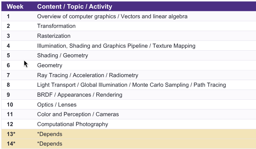
CSC4140 Computer Graphics
L1 Course Introduction
Recommend Textbook: Fundamentals of Computer Graphics, 4th Edition — Marschner & Shirley et al., CRC Press
What is Computer Graphics?
Computers: accept, process, transform, and present information.
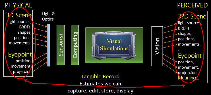
Computer Graphics: the communication channel between the physical world and the digital world.
Why Study Computer Graphics?
History and Applications...
Fundamental Intellectual Challenges:
- Creates and interacts with realistic visual worlds.
- Requires understanding of all aspects of the physical world.
- Demands new computing methods, displays and technologies.
Technical Challenges:
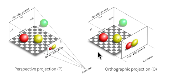
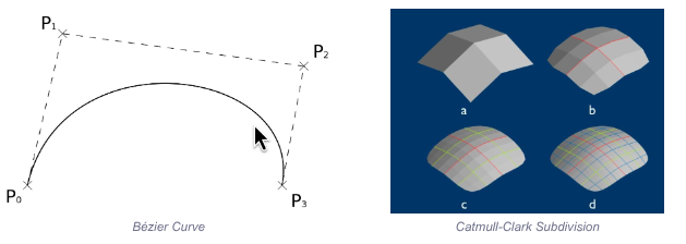
- Math of (perspective) projections, curves and surfaces.
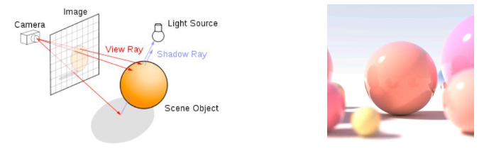
- Physics of lighting and shading.
- Representing / operating on shapes in 3D.
- Animation / simulation.
- Computational photograpy.
Course Topics
Rasterization 光栅化
Curves and Meshes 曲线和网格
Ray Tracing 光线追踪
Animation / Simulation
Computational Photography
Course Logistics
L2 Review of Vectors and Linear Algebra
Linear Algebra
Why Linear Algebra?
Effective bridge between geometry, physics and computation. We can express the solution to a problem in terms of linear algebra, and fasten the calculation speed.
Linear algebra is the study of vector spaces and linear maps between them.
Vectors
This part are mostly learnt at Year 1 UG course, so just a quick review.
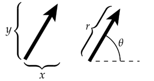
2 Forms of Representing Vectors in 2D:
- Litter Arrow: using $(x,y)$.
- Direction + Magnitude: $(\theta, r)$
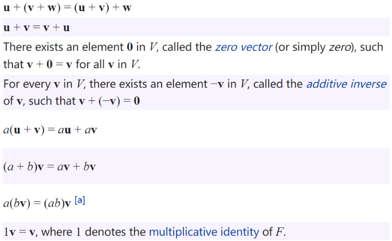
Simple Rules
Cross Product, Determinant and Angle
Useful abuse of notation in 2D.
$$ \sqrt{\det(u, v, u \times v)} = |u| |v| \sin(\theta) $$
where $\theta$ is the angle between $u$ and $v$, $\det$ is the determinant of three column vectors.
Matrices
In graphics, matrices are pervasively used to represent transformations: translation, rotation, shear, scale.
Matrix Representation of Cross Product
Consider a vector:
$$ u := (u_1, u_2, u_3) $$
and we have
$$ \hat{u} := \begin{bmatrix} 0 & -u_3 & u_2 \\ u_3 & 0 & -u_1 \\ -u_2 & u_1 & 0 \end{bmatrix} $$
then
$$ u \times v = \hat{u}v = \begin{bmatrix} 0 & -u_3 & u_2 \\ u_3 & 0 & -u_1 \\ -u_2 & u_1 & 0 \end{bmatrix} \begin{bmatrix} v_1 \ v_2 \ v_3 \end{bmatrix} $$
Notice that
$$ u \times v = -v \times u $$
and we have
$$ v \times u = - \hat{u}v = \hat{u}^\top v $$
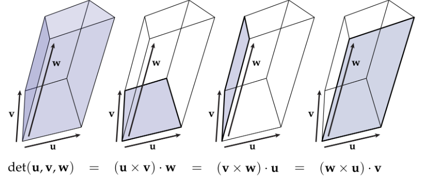
Determinant, Volumn and Triple Product
$\det(u,v,w)$ encodes the (signed) volumn of the parallelepiped with edge vectors $u,v,w$.
Other Triple Products
Jacobi Identity
$$ u \times (v \times w) + v \times (w \times u) + w \times (u \times v) = 0 $$
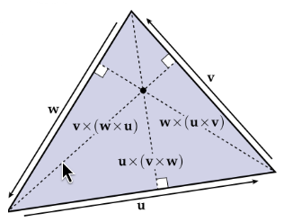
Lagrange's Identity
$$ u \times (v \times w) = v(u \cdot w) - w(u \cdot v) $$
Basis Transformations
Basis Transformations - Formula
Given vector $v$ written in the standard basis, rewrite as $v_Q$ in terms of basis $Q$.
If the columns of $Q$ are orthonormal:
$$ v_Q = Q^\top v $$
Otherwise ($Q$ Not orthonoraml):
$$ v_Q = (Q^\top Q)^{-1} Q^\top v $$
And a useful fact is that: Any matrix of the form $A^\top A$ is positive semi-definite:
$$ x^\top (A^\top A) x = (x^\top A^\top)(Ax)=(Ax)^\top(Ax) \ge 0 $$
Since it is written as a vector dotted with itself, $(Ax)^\top(Ax)$ can never be negative.
Determinants and Rank
Eigenvalues and Eigenvectors
Solving $Ax=b$
Gradient Descent
Steepest Descent
L3 Transformation
Condition Number
For a linear system $Ax=b$, obviously $x=A^{-1}b$. Apply a small perturbation $\delta$: $A(x+\delta)=b+\delta$, that is adding an error in $x$, we can get the relative error in $b$:
$$ \frac{\Vert A^{-1} \delta \Vert}{\Vert A^{-1} b \Vert} \quad \text{v.s.} \quad \frac{\Vert \delta \Vert}{\Vert b \Vert} $$
Consider:
$$ \begin{aligned} & \max \left( \frac{\Vert A^{-1} \delta \Vert}{\Vert A^{-1} b \Vert} / \frac{\Vert \delta \Vert}{\Vert b \Vert} \right) \\ = & \max \left( \frac{\Vert A^{-1} \delta \Vert}{\Vert \delta \Vert} \times \frac{\Vert b \Vert}{\Vert A^{-1} b \Vert} \right) \\ = & \max \left( \frac{\Vert A^{-1} \delta \Vert}{\Vert \delta \Vert} \times \frac{\Vert Ax \Vert}{\Vert x \Vert} \right) \\ = & \Vert A^{-1} \Vert \times \Vert A \Vert \\ = & \text{Cond}(A) \end{aligned} $$
Condition Number of a function measures how much the output can change for a small change in the input.
$$ \sigma_n = \max \left( \frac{\Vert Ax \Vert}{\Vert x \Vert} \right), \sigma_1 = \min \left( \frac{\Vert Ax \Vert}{\Vert x \Vert} \right) $$
Properties:
- For any matrix $A$, $\text{Cond}(A) \ge 1$
- For the identity matrix $I$, $\text{Cond}(I) = 1$
- For any matrix $A$ and nonzero scalar $c$, $\text{Cond}(cA) = \text{Cond}(A)$
- For any diagonal matrix $D=\text{diag}(d_i)$, $\text{Cond}(D) = \frac{\max \vert d_i \vert}{\min \vert d_i \vert}$
Transformations in CG
Modeling:
- Define shapes in convenient coordinates
- Enable multiple copies of the same object
- Efficiently represent hierarchical scenes
Viewing:
- World coordinates to camera coordinates
- Parallel / perspective projections from 3D to 2D
Transformation (Matrices and Linear)
Translation: $$ x' = x+t_x \quad y' = y+t_y $$

Scale: $$ x' = sx \quad y' = sy $$
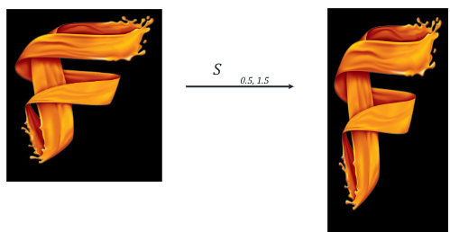
Shear: $$ x' = x+ay \quad y' = y $$

Rotation: $$ R \theta = [\cos \theta, -\sin \theta; \sin \theta, \cos \theta] $$

Reflection: $$ \begin{bmatrix} x' \\ y' \end{bmatrix} = \begin{bmatrix} -1 & 0 \\ 0 & 1 \end{bmatrix} \begin{bmatrix} x \\ y \end{bmatrix} $$
Composing Transforms
?
Homogeneous Coordinates
Unfinished